




Volume 207 - Issue 3
How to measure a QT interval
Authors: Kathryn Waddell-Smith, Robert M Gow and Jonathan R Skinner
Med J Aust 2017; 207 (3): 107-110. || doi: 10.5694/mja16.00442
Published online: 7 August 2017
Published online: 7 August 2017
A standard approach in QT measurement improves communication between clinicians
A standard approach in QT measurement improves communication between clinicians
An abnormally prolonged QT interval is associated with an increased risk of sudden cardiac death.1 Some professional bodies recommend national population-based screening programs to detect QT prolongation.2 Familial long QT syndrome (LQTS) may remain undetected because of misdiagnosis (eg, as a seizure disorder)3 or through failure to measure the QT interval correctly.4 Psychiatrists fear the QT prolongation caused by many psychotropic medications,5 and it may also be seen during periods of hypothermia; electrolyte imbalance (such as hypokalaemia, hypomagnesaemia and hypocalcaemia); in the setting of raised intracranial pressure or post-cardiac arrest; with other medications, such as type 1A, 1C and III antiarrhythmic agents; and with antihistamines and macrolide antibiotics.
Yet, despite its importance, research shows that two physicians cannot measure the same QT interval and get the same result; an observation that also includes cardiac electrophysiologists.4,6 There is no universally accepted agreement about how to measure the QT interval, which 12-lead electrocardiogram (ECG) leads to include,7,8 how many beats to measure,9 or which heart rate correction formula to use.9 Two large international familial LQTS registries measure the end of the T wave in different ways, such that one has an average QT interval (454 milliseconds)10 40 milliseconds below the other (494 milliseconds).11 Moreover, the QT interval has been shown to vary minute to minute, beat to beat, and day by day.9,12 Because of these problems, guidance as to how to obtain accurate and reproducible QT measurements is a matter of opinion and experience.
Principles for measuring and assessing the QT interval
Make measurements on a good quality electrocardiogram equipment
Corrected QT (QTc) calculation is prone to error,4 so in ensuring a quality ECG with flat baseline, a minimal artefact with high resolution (not faxed) helps to obtain an accurate measurement. When possible, QTc measurement is best done during stable sinus rhythm. This is because the heart rate changes due to emotional or postural changes; moreover, sinus arrhythmia, ventricular ectopic beats and arrhythmias (such as atrial fibrillation) affect the accuracy of the QTc,13-15 as does the presence of bundle branch block and Wolff–Parkinson–White syndrome16 — in these two cases, specialist measurement of the QT is advised.
In athletes, when the heart rate is less than 50 beats per minute, some light aerobic activity increasing the heart rate to 60–90 beats per minute improves the accuracy of the Bazett correction.17
For uncertain cases, obtain a second or third electrocardiogram
The QT interval varies constantly and under different influences.9,12,18 Therefore, an individual may have a normal or borderline QTc one moment or day, and a prolonged one the next. A repeat ECG on the same day may be helpful, but if there is no urgency, two to three repeat ECGs over a few days or weeks may help in arriving at the correct conclusion in borderline cases.
Manually measure the QT
While the automatic algorithms used to measure the QT interval on commercial ECG machines are mostly accurate, significant measurement errors are not uncommon.15 Likewise, some automatic reporting systems suppress the QT prolongation statement if the heart rate is greater than 100 beats per minute, which is misleading for people who rely on the automatic reports for guidance. Therefore, we recommend manual measurement to the nearest 5 milliseconds (one quarter of a small square)19 and referencing to normal values.20 To increase accuracy, some specialists advocate taking the average QT of three to five consecutive QRS-T complexes from a single lead at a paper speed of 50 mm per second.9,21 This process is time consuming and has not always been done routinely; taking instead the longer of two measurements, one in lead II and one in V5 and using a normal paper speed (ie, 25 mm per second).
Become accustomed to normal T wave appearance and be suspicious of unusual shapes
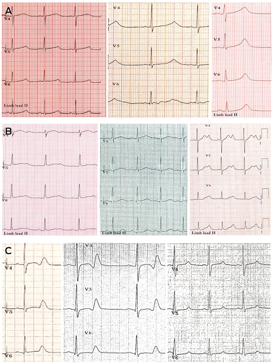
One way to diagnose familial LQTS is with quantitative QTc assessment, when no other QT prolonging influences or medications are present (QTc > 500 milliseconds on two occasions, or > 480 milliseconds with symptoms),1,22 but qualitative T wave assessment is also useful.23 An unusually shaped T wave should raise the suspicion of familial LQTS when other causes are absent. Characteristic T wave findings in the three most common types of LQTS include broad T waves in LQT1, bifid T waves in LQT2 and late onset T waves in LQT323 (Box 1, A, B and C respectively).
Focus on leads II and V5
Measurements are made in leads II and V5 because QTc in these leads correlates best with genotype status in LQTS, either alone or in combination,24 and results are highly repeatable.19 Moreover, a consistent approach is required because T wave projection and noise vary between the leads.8 We use the longer of these two measurements.2
Use the tangent technique
The end of the T wave (which can be difficult to define)7 can be most reproducibly ascertained using the tangent technique, where a line or tangent is drawn down the steepest slope of the terminal limb of the T wave. The end of the T wave is defined by the intersection of this line with the baseline,25 which is measured as the TP or PR segments on a standard ECG,26 or on an exercise test as the QQ line19 (Box 2, A and B respectively).
Be aware of bifid T waves and U waves
Where a T wave is bifid, the second peak should be included if it is at least half the amplitude of the first using the tangent technique (Box 3, A).27 When a U wave is present, if large (ie, > 50% amplitude of the T wave) and merging into the T wave, it should probably be included, but excluded if it is smaller or separate9 (Box 3, B).
Consider referencing neighbouring leads
The end of the T wave may still be difficult to define after using the tangent technique, such as when the T wave is very flat. When this occurs, several approaches are possible. Drawing a vertical line down through the two adjacent leads may help to determine the T wave end; or measuring the QT in a non-traditional lead (such as leads I, III or V6) and taking the longest of these may provide an alternative (Box 4).26 Leads V1–V3 should be avoided, particularly in children and young adults (especially females) where T wave morphology is greatly variable.26
Consider techniques to expose latent QT prolongation in individuals who have first-degree relatives with familial long QT syndrome and a normal or borderline QTc
Up to 30% of individuals with familial LQTS may have QTc intervals within the normal range, and unmasking QTc prolongation may occur with provocative tests.
Standing test
This is a relatively new technique, requiring validation and more normative data (especially in children), but may add diagnostic information if a high pre-test probability of LQTS exists. Record a 12-lead ECG when supine, ask the patient to briskly stand, and record another ECG about 10 seconds later. At this time, a tachycardia has resulted, and in patients with LQTS, the QT does not adapt and shorten to the reduced RR interval as quickly as in people without LQTS. Therefore, the QTc interval increases much more in patients with LQTS than in patients without it. Characteristic LQTS T wave morphology (such as bifid T waves) may also be revealed.28
Exercise test
On formal exercise testing, the QTc intervals of patients with LQTS recorded during the recovery period are usually longer than for non-carrier patients. A post-exercise recovery QTc taken at 4 minutes that exceeds 480 milliseconds29 is supportive evidence of LQTS in adults.30 In children, a highly reproducible technique averages four consecutive QT intervals in lead II (where the end of the T wave is defined as the intersection of the tangent and a baseline of the QQ line; Box 2, B). A QTc equal to or exceeding 500 milliseconds suggests LQTS. Because children’s heart rates recover more slowly than adults’,19,31 consider monitoring another 7 minutes of recovery: a carefully measured average QTc exceeding 470 milliseconds at this point (after a bicycle ergometry test) suggests LQTS.31
Holter monitor
Holter recordings are not yet standard in the diagnosis of LQTS, but are promising. Holter QTc is significantly longer in patients who carry LQTS compared with their gene-negative relatives,32,33 and assessment of morphology34 and other techniques35 may also aid in the diagnosis and genotype identification in the future.
Consider which correction method is most appropriate
There are many correction formulas available, but none are universally applicable, and all have limitations resulting in over- or undercorrection. Despite its flaws, the most commonly used technique (for its simplicity and association with outcome data) is the Bazett formula. Here, the QT (in seconds) is divided by the square root of the preceding RR interval (in seconds).36 The main limitation of this formula is a variable effect on the correction of the absolute QT interval that is dependent on heart rate. In borderline cases, it is wise to take an average of three to five beats for both the QT and RR intervals. The formula produces a shorter QTc at low heart rates and a longer QTc at high heart rates.37 In view of these limitations, consideration may be given to using other correction formulas, although there are few outcome data relating to these, and comparison with relevant reference ranges is required.38 As an example, the Fredericia, Hodges or Framingham formulas may be used, and even genotype-specific formulas exist for QT correction in LQTS types 1 and 2.39
Interpret borderline QTc values in the context of pre-test probability
While overt QTc prolongation may indicate LQTS,1 the interpretation of borderline values is challenging because of the considerable variation in clinical phenotypes,40 and because data from controls are varied.19,31 A borderline result (Box 5) should be interpreted in the context of the pre-test probability: a 12-lead ECG QTc of 450 milliseconds in a person without a family history of LQTS is most likely normal, but in a relative of a patient with LQTS, it probably represents a diagnosis of LQTS. In this situation, calculation of the Schwartz score may be helpful.30
Consider seeking expert advice
This article aims to provide clinicians with techniques to most accurately determine the QTc interval and to monitor the effects of medications. However, because assessment of QTc is so difficult in borderline cases, and values carry such high significance, the involvement of a cardiologist specialised in LQTS may be best.4 Such a physician will usually be found in a cardiac genetics clinic, which is where we advocate that patients with suspected familial LQTS are reviewed.1,22
Conclusion
QT measurement and correction is complex, but a standard approach allows improved communication between clinicians. We would recommend that the QT is measured manually, on at least one good quality ECG machine, in lead II or V5 using the tangent technique, incorporating large bifid T waves and U waves, and corrected with the Bazett formula. In borderline cases, the ECG should be repeated, and techniques considered to help expose latent QT prolongation, such as exercise testing, should be used.
Box 2 – QT correction method on 12-lead ECG (A): measure the QT interval using the tangent technique and the preceding RR interval. QT correction method exercise stress test (B): define the end of the T wave as the intersection of a tangent from the steepest slope of the last limb of the T wave and the baseline.*
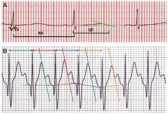
* The baseline is defined as the QQ line to provide a consistent reference for each QT interval. The QT measurement derived from the tangent line is divided by the square root of the previous RR interval (shown by the colour pairs).
Box 3 – Bifid T wave (A), where the second limb is > 50% amplitude of the first and should be included. Prominent U wave (B), which should be excluded
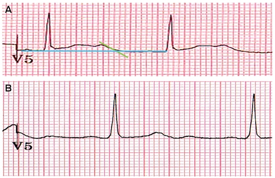
The blue line (A) corresponds to the baseline (QQ line); the green line (A) is the tangent from the TU wave. The end of the TU wave is defined by the point where the green line crosses the blue line.
Box 4 – Dropping a vertical line (dotted lines) down through several leads may help determine the T wave end
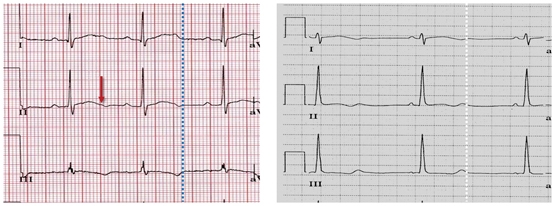
The arrow points to the place where the T wave appears to end in this lead. However, by drawing a vertical line between neighbouring leads I and III, it is clear that the negative deflection here should be included in the T wave.
Box 5 – Borderline result interpreted in the context of the pre-test probability
|
|
Men |
Women |
Children |
||||||||||||
|
|
|||||||||||||||
|
QTc diagnostic of LQTS |
> 500 ms |
> 500 ms |
> 500 ms |
||||||||||||
|
(> 480 ms with symptoms) |
(> 480 ms with symptoms) |
(> 480 ms with symptoms) |
|||||||||||||
|
Prolonged QTc |
> 450 ms |
> 470 ms |
> 460 ms |
||||||||||||
|
Borderline QTc |
430–450 ms |
450–470 ms |
440–460 ms |
||||||||||||
|
Normal QTc |
< 430 ms |
< 450 ms |
< 440 ms |
||||||||||||
|
|
|||||||||||||||
|
LQTS = long QT syndrome. MS = milliseconds. QTc = corrected QT. |
|||||||||||||||
Competing interests
Jon Skinner has no relevant disclosures. Kathryn Waddell-Smith is supported by grants from the Green Lane Research and Educational Fund and the National Heart Foundation, New Zealand.
References
- Priori SG, Wilde AA, Horie M, et al. HRS/EHRA/APHRS expert consensus statement on the diagnosis and management of patients with inherited primary arrhythmia syndromes: document endorsed by HRS, EHRA, and APHRS in May 2013 and by ACCF, AHA, PACES, and AEPC in June 2013. Heart Rhythm 2013; 10: 1932-1963.
- Earle N, Crawford J, Smith W, et al. Community detection of long QT syndrome with a clinical registry: an alternative to ECG screening programs? Heart Rhythm 2013; 10: 233-238.
- MacCormick JM, McAlister H, Crawford J, et al. Misdiagnosis of long QT syndrome as epilepsy at first presentation. Ann Emerg Med 2009; 54: 26-32.
- Viskin S, Rosovski U, Sands AJ, et al. Inaccurate electrocardiographic interpretation of long QT: the majority of physicians cannot recognize a long QT when they see one. Heart Rhythm 2005; 2: 569-574.
- Wenzel-Seifert K, Wittmann M, Haen E. QTc prolongation by psychotropic drugs and the risk of Torsade de Pointes. Dtsch Arztebl Int 2011; 108: 687-693.
- Taggart NW, Haglund CM, Tester DJ, et al. Diagnostic miscues in congenital long-QT syndrome. Circulation 2007; 115: 2613-2620.
- Lepeschkin E, Surawicz B. The measurement of the Q-T interval of the electrocardiogram. Circulation 1952; 6: 378-388.
- Malik M. Beat-to-beat QT variability and cardiac autonomic regulation. Am J Physiol Heart Circ Physiol 2008; 295: H923-H925.
- Anderson ME, Al-Khatib SM, Roden DM, et al. Cardiac repolarization: current knowledge, critical gaps, and new approaches to drug development and patient management. Am Heart J 2002; 144: 769-781.
- Hofman N, Wilde AA, Kaab S, et al. Diagnostic criteria for congenital long QT syndrome in the era of molecular genetics: do we need a scoring system? Eur Heart J 2007; 28: 575-580.
- Hobbs JB, Peterson DR, Moss AJ, et al. Risk of aborted cardiac arrest or sudden cardiac death during adolescence in the long-QT syndrome. JAMA 2006; 296: 1249-1254.
- Morganroth J, Brozovich FV, McDonald JT, et al. Variability of the QT measurement in healthy men, with implications for selection of an abnormal QT value to predict drug toxicity and proarrhythmia. Am J Cardiol 1991; 67: 774-776.
- Tutar HE, Ocal B, Imamoglu A, et al. Dispersion of QT and QTc interval in healthy children, and effects of sinus arrhythmia on QT dispersion. Heart 1998; 80: 77-79.
- Postema PG, Wilde AA. The measurement of the QT interval. Curr Cardiol Rev 2014; 10: 287-294.
- Malik M. Errors and misconceptions in ECG measurement used for the detection of drug induced QT interval prolongation. J Electrocardiol 2004; 37 Suppl: 25-33.
- Talbot S. QT interval in right and left bundle-branch block. Br Heart J 1973; 35: 288-291.
- Drezner JA, Ackerman MJ, Cannon BC, et al. Abnormal electrocardiographic findings in athletes: recognising changes suggestive of primary electrical disease. Br J Sports Med 2013; 47: 153-167.
- Funck-Brentano C, Jaillon P. Rate-corrected QT interval: techniques and limitations. Am J Cardiol 1993; 72: 17B-22B.
- Berger WR, Gow RM, Kamberi S, et al. The QT and corrected QT interval in recovery after exercise in children. Circ Arrhythm Electrophysiol 2011; 4(4): 448-455.
- Drew BJ, Califf RM, Funk M, et al. Practice standards for electrocardiographic monitoring in hospital settings: an American Heart Association scientific statement from the Councils on Cardiovascular Nursing, Clinical Cardiology, and Cardiovascular Disease in the Young: endorsed by the International Society of Computerized Electrocardiology and the American Association of Critical-Care Nurses. Circulation 2004; 110: 2721-2746.
- Moss AJ. Measurement of the QT interval and the risk associated with QTc interval prolongation: A review. Am J Cardiol 1993; 72: 23B-25B.
- Waddell-Smith KE, Skinner JR; members of the CSANZ Genetics Council Writing Group. Update on the diagnosis and management of familial long QT syndrome. Heart Lung Circ 2016; 25: 769-776.
- Zhang L, Timothy KW, Vincent GM, et al. Spectrum of ST-T-wave patterns and repolarization parameters in congenital long-QT syndrome: ECG findings identify genotypes. Circulation 2000; 102: 2849-2855.
- Monnig G, Eckardt L, Wedekind H, et al. Electrocardiographic risk stratification in families with congenital long QT syndrome. Eur Heart J 2006; 27: 2074-2080.
- Postema PG, De Jong JS, Van der Bilt IA, et al. Accurate electrocardiographic assessment of the QT interval: teach the tangent. Heart Rhythm 2008; 5: 1015-1018.
- Rautaharju PM, Surawicz B, Gettes LS, et al. AHA/ACCF/HRS recommendations for the standardization and interpretation of the electrocardiogram: part IV: the ST segment, T and U waves, and the QT interval: a scientific statement from the American Heart Association Electrocardiography and Arrhythmias Committee, Council on Clinical Cardiology; the American College of Cardiology Foundation; and the Heart Rhythm Society. Endorsed by the International Society for Computerized Electrocardiology. J Am Coll Cardiol 2009; 53: 982-991.
- Goldenberg I, Moss AJ, Zareba W. QT interval: how to measure it and what is “normal”. J Cardiovasc Electrophysiol 2006; 17: 333-336.
- Viskin S, Postema PG, Bhuiyan ZA, et al. The response of the QT interval to the brief tachycardia provoked by standing: a bedside test for diagnosing long QT syndrome. J Am Coll Cardiol 2010; 55: 1955-1961.
- Sy RW, van der Werf C, Chattha IS, et al. Derivation and validation of a simple exercise-based algorithm for prediction of genetic testing in relatives of LQTS probands. Circulation 2011; 124: 2187-2194.
- Schwartz PJ, Crotti L. QTc behavior during exercise and genetic testing for the long-QT syndrome. Circulation 2011; 124: 2181-2184.
- Aziz PF, Wieand TS, Ganley J, et al. Genotype- and mutation site-specific QT adaptation during exercise, recovery, and postural changes in children with long-QT syndrome. Circ Arrhythm Electrophysiol 2011; 4: 867-873.
- Kaufman ES, Priori SG, Napolitano C, et al. Electrocardiographic prediction of abnormal genotype in congenital long QT syndrome: experience in 101 related family members. J Cardiovasc Electrophysiol 2001; 12: 455-461.
- Mauriello DA, Johnson JN, Ackerman MJ. Holter monitoring in the evaluation of congenital long QT syndrome. Pacing Clin Electrophysiol 2011; 34: 1100-1104.
- Vaglio M, Couderc JP, McNitt S, et al. A quantitative assessment of T-wave morphology in LQT1, LQT2, and healthy individuals based on Holter recording technology. Heart Rhythm 2008; 5: 11-18.
- Page A, Aktas MK, Soyata T, et al. “QT clock” to improve detection of QT prolongation in long QT syndrome patients. Heart Rhythm 2016; 13: 190-198.
- Bazett H. An analysis of the time relations of electrocardiograms. Heart 1920; 7: 353-370.
- Milne JR, Ward DE, Spurrell RA, et al. The ventricular paced QT interval–the effects of rate and exercise. Pacing Clin Electrophysiol 1982; 5: 352-358.
- Rijnbeek PR, van Herpen G, Bots ML, et al. Normal values of the electrocardiogram for ages 16-90 years. J Electrocardiol 2014; 47: 914-921.
- Barsheshet A, Peterson DR, Moss AJ, et al. Genotype-specific QT correction for heart rate and the risk of life-threatening cardiac events in adolescents with congenital long-QT syndrome. Heart Rhythm 2011; 8: 1207-1213.
- Vincent GM, Timothy KW, Leppert M, et al. The spectrum of symptoms and QT intervals in carriers of the gene for the long-QT syndrome. N Engl J Med 1992; 327: 846-852.
Provenance: Commissioned; externally peer reviewed.
Newborn Screening: Equity for Aboriginal and Torres Strait Islander Families in the Context of Emerging Genomics
Gail Garvey, Sarah Norris, Joanne Scarfe, Louise Lyons
When ‘Liver Enzymes’ Are Not Hepatic: Late-Onset Pompe Disease
Shauna Madigan, Georgina England, Wayne Rankin
Genomic Newborn Screening: Verdict From an Australian Citizens’ Jury
Emma Frost, Zornitza L. Stark, Kristen Nowak, Louise Healy, Sarah Norris, Stacy M. Carter
Genomic Testing Access for Hearing Loss Must Catch Up to the Evidence
Emma McGonigal, Andrew V. White, Valerie Sung, Karen Liddle, Lilian Downie, Emily Shepard
Population-Based Melanoma Screening Using Integrated Risk Scores in Australia: A Narrative Review to Determine Readiness
Courtney K. Wallingford, Chloe Mighton, Tamara Dawson, Anne Cust, H. Peter Soyer, Yvonne Bombard, Tatiane Yanes, Aideen McInerney-Leo
Genomic Newborn Screening: Commodity or Public Good?
Christopher Gyngell, Sebastian Lunke, Danya Vears, Zornitza L. Stark