Standard deviation and standard error: interpretation, usage and reporting

Standard deviations (SDs) and standard errors are reported routinely in statistical analyses, but the distinction between them is not always well understood.1,2 Incorrect and also unclear reporting of results adds to the potential for confusion and misinterpretation of these measures.3,4

SD describes the variability between individual observations about their mean value. It is rarely possible to obtain measurements for all members of a population, so we estimate the population mean (usually denoted by μ) and the population SD (σ) using the mean and SD of a random sample of observations drawn from that population. The greater the spread of the observations about the mean, the larger the SD.

The mean and SD are used to describe a distribution. For example, the diastolic blood pressure response to 4 weeks of hydrochlorothiazide (25 mg/day) was measured in a sample of 505 men and women with hypertension.5 A mean decrease of 7.8 mmHg was observed over the 4-week period, with an SD of 8.4 mmHg. A histogram provided in the publication indicates that the change in diastolic blood pressure is approximately normally distributed, so we would expect about 95% of the population from which this sample was drawn to have a change in diastolic blood pressure within 1.96 SD units above and below the mean (ie, −7.8 ± 1.96 × 8.4 = −24.3 to 8.7 mmHg) if they undergo the same treatment. This range indicates the level of variability between individuals in their response to therapy.

Even though the SD can be calculated for any sample, alternative summary measures based on percentiles (median and interquartile range) are often reported to describe non-normal distributions. This is commonly done for skewed distributions, where the 5% of observations expected to fall outside the range given by 1.96 SD units above and below the mean will not be equally split between the two tails of the distribution.1 Graphical displays such as histograms provide a useful tool to visualise the shape of a distribution.

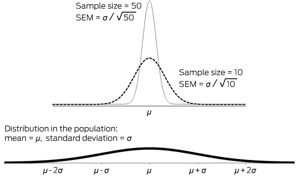
The standard error of the mean (SEM, often abbreviated as SE) estimates the statistical uncertainty associated with the mean estimated from a sample. The study sample is only one of the possible samples of the same size (n) that could have been selected by chance from the population, and the observed sample mean will vary between these alternative hypothetical samples. The distribution of these hypothetical sample means is referred to as the sampling distribution of the mean, and the SEM is a measure of the variability between the (hypothetical) sample means in the sampling distribution. Intuitively, we would expect the mean estimated from a large sample to be more precise (ie, closer on average to the true population mean μ) than an estimate from a small sample. The SEM is computed as σ/√n, where the underlying population SD (σ) is estimated by the sample SD. The formula includes the sample size in the denominator, which means that the SEM will decrease as n increases. Box 1 illustrates how the variability between the sample means decreases as the sample size increases from 10 to 50, resulting in improved precision. The SEM is never larger than the SD.

In Box 1, the underlying population distribution is assumed to be normal. As the sample size (n) increases, the sampling distribution of the mean will usually approximate a normal distribution, irrespective of the underlying distribution of individual observations (central limit theorem). This property of sampling distributions allows inferences to be made not only for a mean but also for other population parameters that are estimated from a sample (eg, a proportion, difference between means and difference between proportions).

The SEM is used to calculate a confidence interval around the estimated mean6 and to calculate a P value when testing a hypothesis.7 In our example, the sample size (n) is 505 and SD is 8.4 mmHg giving an SEM=8.4/√505=0.37mmHg. The confidence interval is centred on the sample mean (−7.8 mmHg), which is our estimate of the unknown population mean (μ), and the 95% confidence limits are computed as −7.8 ± 1.96 × 0.37. Hence, we are 95% confident that the true underlying average diastolic blood pressure response in the population is a reduction of between 7.1 and 8.5 mmHg.

Systematic investigations of the frequency of inappropriate reporting and interpretation of the SD and SEM have been undertaken. A review of articles published in four anaesthesia journals in 20013 identified that 23% (198/860) of the included articles had inappropriately used the SEM (instead of the SD) in descriptive analyses to quantify the variability between individuals in the study sample. A more recent review of publications that appeared in three cardiovascular journals in 20124 reported that the methods section included an explicit statement on using SEM for description of the data in 52% (228/441) of the included articles. The inappropriate use of the SEM was highest in the two journals where over 90% of articles were from laboratory or basic sciences.3,4

It is common, particularly in laboratory and basic sciences, for authors to report the sample mean ± SD (or ± SEM). The use of the ± notation is ambiguous if adequate labelling is not used in the text and tables, leading to confusion about whether it is the SD or the SEM that is being referred to (Box 2). The methods section may provide the necessary information in some articles, but not in all.4 The incorrect use of the SEM to describe the sample data underestimates the variability between individuals. In our example, the large sample size has resulted in a small SEM of 0.37 mmHg. Using the SEM instead of the SD (= 8.4 mmHg) to describe the variability between individuals in their response to therapy would be grossly misleading.

Box 1 – Sampling distributions of means for n = 10 and n = 50

---

SEM = standard error of the mean.

References

- Altman DG, Bland JM. Standard deviations and standard errors. BMJ 2005; 331: 903.
- Biau DJ. In brief: standard deviation and standard error. Clin Orthop Relat Res 2011; 469: 2661-2664.
- Nagele P. Misuse of standard error of the mean (SEM) when reporting variability of a sample. A critical evaluation of four anaesthesia journals. Br J Anaesth 2003; 90: 514-516.
- Wullschleger M, Aghlmandi S, Egger M, Zwahlen M. High incorrect use of the standard error of the mean (SEM) in original articles in three cardiovascular journals evaluated for 2012. PLoS One 2014; 9: 1-4.
- Chapman AB, Schwartz GL, Boerwinkle E, Turner ST. Predictors of antihypertensive response to a standard dose of hydrochlorothiazide for essential hypertension. Kidney Int 2002; 61: 1047-1055.
- Carlin JB, Doyle LW. Basic concepts of statistical reasoning: standard errors and confidence intervals. J Paediatr Child Health 2000; 36: 502-505.
- Carlin JB, Doyle LW. Basic concepts of statistical reasoning: hypothesis tests and the t-test. J Paediatr Child Health 2001; 37: 72-77.
Provenance: Commissioned; externally peer reviewed.
Interpreting Australian Stillbirth Rate Trends: Implications for Surveillance and Continuous Quality Improvement
Aleena M. Wojcieszek, Kirstine Sketcher-Baker, Christine Andrews, Michael Coory, Imogen Kettle, Melissa Malivoire, David Ellwood, Vicki Flenady
Paracetamol in Pregnancy: Uncertain Evidence, Certain Consequences
David J. Tunnicliffe, Miranda Cumpston, Debra Kennedy, Margie Danchin, Armando Teixeira-Pinto
Fatty Liver Disease in Australia: A Narrative Review on the Epidemiology, Natural History, Prognostication and Management in People With Metabolic Dysfunction
Karl Vaz, Daniel Clayton-Chubb, William W. Kemp, Stuart K. Roberts, Ammar Majeed
Birth prevalence, clinical sequelae, and management of congenital cytomegalovirus infections in Australia, 1999–2023: a national prospective study
Ece Egilmezer, Suzy M Teutsch, Carlos Nunez, Stuart T Hamilton, Adam W Bartlett, Pamela Palasanthiran, Elizabeth J Elliott, William D Rawlinson
The number of cancer‐related deaths that could be attributable to spatial disparities in survival in Australia, 2010–2019: a retrospective population‐based cohort study
Charlotte K Bainomugisa, Jessica Cameron, Paramita Dasgupta, Peter Baade
Mandatory research projects during medical specialist training in Australia and New Zealand
Paulina Stehlik, Caitlin Brandenburg, David A Henry