Guided by the research design: choosing the right statistical test

Choosing the right statistical test or model can be baffling for researchers, and if it is not conducted correctly, the results from statistical analyses can be misleading. This article covers some common medical research designs, ranging from simple to more complicated, and provides an outline of which statistical test to apply in each instance. In these contexts, data are collected from a sample that is assumed to be representative of a wider population, and the conclusions drawn from the analyses apply to the wider population.1

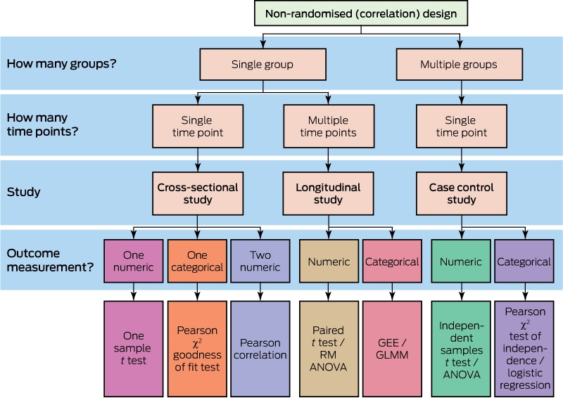
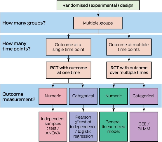
This article follows the process outlined in decision trees (Box 1 and Box 2), which describe the conditions under which a particular test is appropriate, that is:

• the type of research design (non-randomised in Box 1 v randomised in Box 2);

• whether group comparisons are being made or a single population is of interest;

• whether an outcome is measured once or repeatedly over time; and

• whether the outcome variable is on a numeric or categorical measurement scale.

Each of the tests discussed can be used for purposes beyond the ones covered here; however, the aim of this article is to outline which test is appropriate to use for each design, not to discuss all possible variations and extensions of the tests themselves. Throughout the article, the tests are set inside the particular research context (Box 1 and Box 2), and more detail is provided for more complex statistical models. In addition, the online Appendix includes an example research question to correspond with each design and test.

Non-randomised (correlational) design

Non-randomised designs involve no random allocation to groups, treatments or conditions; the researcher collects data from subjects at either a single time point (eg, cross-sectional study) or repeated time points (eg, longitudinal or cohort study). Any groupings are naturally occurring. The lack of any experimental control means that cause and effect conclusions should only be drawn with great caution, and often they are not feasible due to placebo effects in addition to confounding due to common cause. Any potentially confounding influences also need consideration.

Cross-sectional study

A cross-sectional study collects data from a single point in time.

• One-sample Student t test. This test is used for a single (numeric) variable of interest to compare the mean score of this variable with a known (external) reference score, such as the mean of a different population.

• Pearson χ²  goodness of fit test. This test is used for a single (categorical) variable of interest to compare the proportion of observations across categories with some known reference proportions, such as those of a different population.

• Pearson correlation. It is used to test the association between two (numeric) variables; specifically, the linear relationship, positive or negative. As an extension, a partial correlation can estimate the strength of the association, holding constant or controlling for one or more covariates (potentially confounding variables). This is particularly common in non-randomised research designs, when potential confounding variables are often present.

Longitudinal study

A longitudinal study collects multiple measurements from the same individuals over time. These studies are typically designed to investigate the change in an outcome over time, within the non-randomised research framework; that is, without random allocation to treatment conditions. For reference, one type of longitudinal study is a cohort study.

• Paired Student t test or repeated measures analysis of variance (ANOVA). These are used for numeric outcomes to test whether the mean score on a (numeric) measure changes over time (two or more time points). A paired t test compares the score over two time points only, and the repeated measures ANOVA fits a model testing whether the numeric outcome changes over any number of time points. Three or more time points allow more specific hypotheses to be tested using contrast testing (eg, does Time 1 differ from Time 2? Does Time 1 differ from the mean of Times 2 and 3?); alternatively, polynomial trends (eg, linear or quadratic shape changes) can be tested. Both of these models test a single effect, the time effect, with two or more levels.

• Generalised estimating equations (GEE) or generalised linear mixed model (GLMM). These tests can be used for categorical outcomes, to test whether the proportion of observations across categories change over time (two or more time points). GEE and GLMM are broadly similar, both capable of analysing categorical repeated measures data, but mathematically different.2,3 For this research design, there is a single effect of interest in these models: the time effect (with as many levels as there are time points). In addition, hypotheses about the specific change over time can be tested using contrast testing.

Case–control study

Case–control studies typically investigate a particular clinical population, examining differences between the clinical cases and an appropriate control group, which may be matched to the clinical cases on relevant characteristics (eg, age, weight, etc). Cases are typically patients with a targeted disease and controls are typically people who do not have the condition. Here, the outcome is measured at a single point in time.

• Independent samples Student t test or ANOVA. These tests can be used to compare the mean score on a (numeric) measure between two or more groups (a clinical case group and a control group, or multiple clinical groups and a control group). The independent samples t test is restricted to comparisons of two groups only, whereas with ANOVA, group differences are tested using contrasts (eg, is Group 1 different to Group 2? Is Group 3 different to the mean of Groups 1 and 2?). The model is investigating a single effect: the group effect. As an extension, analysis of covariance (ANCOVA) models can be used to address research questions of between-group differences where potentially confounding variables (covariates) are included in the model to control for their effect, such as a non-matched case–control study.

• Pearson χ²  test of independence or logistic regression. This is used to compare the clinical case group and control group (or multiple clinical groups and a control group) on a categorical outcome; for example, to assess the likelihood of a secondary disease or medical problem. There is a single effect of interest in this model: the group effect (ie, comparison of clinical group and control group on the outcome). The χ²  test and logistic regression are fitting the same kind of model to the data, but the logistic regression also can be used to fit a more complex model, such as an ANCOVA-type model if there were factors that the groups were not matched on, to control for potential confounding variables. If cases and controls are not matched, χ²  tests and unconditional logistic regression models should be used. If groups are matched, conditional logistic regression models should be used.

Randomised (experimental) designs

Randomised designs differ fundamentally from non-randomised designs by having experimental control: subjects are randomly allocated to independent groups (conditions). Because of this random allocation (eg, experimental group v control group in a randomised control trial), cause and effect conclusions can be drawn, as there is very little chance of differences between the groups other than the condition of the study, and even this small possibility can be evaluated, therefore leaving little potential for confounding variables.

Randomised controlled trial with a single point in time endpoint

The independent samples Student t test and ANOVA as well as the χ²  test or logistic regression can be used as described above.

Randomised controlled trial with repeated measurement outcomes

The difference between this and the previous randomised controlled trial is the addition of multiple outcome measurements over time, typically used to test the long term efficacy of the treatment or intervention.

• General linear mixed model. It is used to understand how a numeric outcome changes over time, and whether that change varies across two (or more) groups. The general linear mixed model takes into account the time effect (with two or more levels), the effect of group (with two or more levels), plus a third effect, which tests how the effect of time is modified by group (ie, how the change over time differs between groups), represented by a statistical interaction between the time effect and the group effect.4 As outlined previously, three or more groups allow for specific hypotheses to be tested using contrasts (eg, whether the change over time is more pronounced in Group 3 v Groups 1 and 2).

• Generalised estimating equations or generalised linear mixed model. They are used to test whether the proportion of subjects who experience an outcome change over time and if this change varies across (independent) groups. The GEE and GLMM models are the same as discussed previously, but with the addition of some other statistical effects in the model, such as the general linear mixed model. Here, there is an effect of time (with two or more levels), effect of group (with two or more levels), plus the effect we are interested in (ie, how the change over time of the outcome differs between groups) as a statistical interaction between the time effect and the group effect.

Additional considerations

The types of study design covered in this article include those commonly used in medical research. Readers may also come across more complex sampling schemes, such as multilevel or cluster sampling, often used in health surveys, which require particular statistical adjustments for the fact that observations are not completely independent (eg, observations are usually more related within a particular cluster than across different clusters).1 These adjustments can be made within the framework of mixed or multilevel model,5 but a detailed treatment is beyond the scope of this article.

Every statistical hypothesis test has a statistical model underlying it. When interpreting the model, we interpret both a significance test (eg, Student t test) and a measure of effect size (eg, magnitude of the difference between groups). Many different types of effect size can be calculated and are typically chosen to suit the statistical model and measurement scale of the data: between-group differences in a numeric outcome can be illustrated by Cohen’s d or ε², and group differences in categorical outcomes can be illustrated by a relative risk or odds ratio. The magnitude of the effect is arguably more clinically meaningful than the results of the significance test.6

Conclusions

In summary, there are clear conditions under which certain tests are appropriate (Box 1 and Box 2):

• what is the research design (randomised or non-randomised)?

• are group comparisons being made?

• is the outcome measured once or repeatedly over time? and

• what is the measurement scale of the outcome?

While these individual tests might seem distinct, there is a common framework that connects them all: the generalised linear model.7 All these models are used for a common aim, to understand or predict variation in an outcome and have a common formula to define their models.

Box 1 – Decision tree for non-randomised study designs

---

ANOVA = analysis of variance. GEE = generalised estimating equations. GLMM = generalised linear mixed model. RM = repeated measures.

Box 2 – Decision tree for randomised study designs

---

ANOVA = analysis of variance. GEE = generalised estimating equations. GLMM = generalised linear mixed model. RCT = randomised controlled trial.

References

- Jones MP, Attia JR. Sampling: how you choose people is as important as how you analyse their data. Med J Aust 2017; 206: 67-68.
- Lindsey JK, Lambert P. On the appropriateness of marginal models for repeated measurements in clinical trials. Stat Med 1998; 17: 447-469.
- Hubbard AE, Ahern J, Fleischer NL, et al. To GEE or not to GEE: comparing population average and mixed models for estimating the associations between neighborhood risk factors and health. Epidemiology 2010; 21: 467-474.
- Cnaan A, Laird N, Slasor P. Using the general linear mixed model to analyse unbalanced repeated measures and longitudinal data. Stat Med 1997; 16: 2349-2380.
- Goldstein H. Multilevel mixed linear model analysis using iterative generalized least squares. Biometrika 1986; 73: 43-56.
- Sullivan GM, Feinn R. Using effect size — or why the P value is not enough. J Grad Med Educ 2012; 4: 279-282.
- Dobson AJ, Barnett A. An introduction to generalized linear models; 3rd ed. Boca Raton, FL: CRC Press; 2008.
Provenance: Commissioned; externally peer reviewed.
Interpreting Australian Stillbirth Rate Trends: Implications for Surveillance and Continuous Quality Improvement
Aleena M. Wojcieszek, Kirstine Sketcher-Baker, Christine Andrews, Michael Coory, Imogen Kettle, Melissa Malivoire, David Ellwood, Vicki Flenady
Paracetamol in Pregnancy: Uncertain Evidence, Certain Consequences
David J. Tunnicliffe, Miranda Cumpston, Debra Kennedy, Margie Danchin, Armando Teixeira-Pinto
Fatty Liver Disease in Australia: A Narrative Review on the Epidemiology, Natural History, Prognostication and Management in People With Metabolic Dysfunction
Karl Vaz, Daniel Clayton-Chubb, William W. Kemp, Stuart K. Roberts, Ammar Majeed
Birth prevalence, clinical sequelae, and management of congenital cytomegalovirus infections in Australia, 1999–2023: a national prospective study
Ece Egilmezer, Suzy M Teutsch, Carlos Nunez, Stuart T Hamilton, Adam W Bartlett, Pamela Palasanthiran, Elizabeth J Elliott, William D Rawlinson
The number of cancer‐related deaths that could be attributable to spatial disparities in survival in Australia, 2010–2019: a retrospective population‐based cohort study
Charlotte K Bainomugisa, Jessica Cameron, Paramita Dasgupta, Peter Baade
Mandatory research projects during medical specialist training in Australia and New Zealand
Paulina Stehlik, Caitlin Brandenburg, David A Henry