Survival studies: competing risks, immortality and censoring

One of the simplest study designs is giving participants — with a headache, for example — an active pill or placebo at random and then observing their outcome of cured or not cured one hour later. Studies with such short time frames are rare, and meaningful outcomes, such as disease or death, often need to be followed up long after the initial contact, potentially decades later.

If time is an integral part of a study, then a key issue is what else happened to the participants during the time between their recruitment and the time at which we tried to record their outcomes. If we did not find them, is that because they emigrated or died? If they died, was their death related to their original illness? Did they take some other therapy in the interim? Time complicates all studies, but most complications can be managed by collecting detailed data on participants over time and using survival analysis.1

Survival analysis

We can use survival analysis to model the time to any important outcome, such as time of relapse or remission, not just death. If we look at the example of smoking and dementia used in previous articles in this series,1-3 we might follow all smokers and non-smokers in a practice from their first general practitioner visit until first diagnosis of dementia. We might also collect data on other potential confounders or predictors, such as age, pack-year history of smoking, education and socio-economic status.

We could create the binary variable of dementia (yes/no) and use logistic regression or a χ² test, but there are problems with this approach. First, we need to account for the time at risk. A smoker who has reached the age of 50 years without dementia is not similar to a smoker who has reached the age of 80 years without dementia, but a binary analysis would treat them both as simply “no”. Second, by simplifying continuous times to binary, we lose information and hence statistical power; for example, if the same number of people end up developing dementia by 90 years of age but smoking accelerates the onset so that smokers spend more follow-up time with dementia, this difference would be harder to find using logistic regression compared with survival analysis.

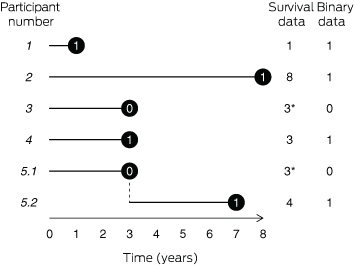
What should we do with smokers who have reached the age of 50 without developing dementia and are lost to follow-up? Should we drop them because they are too young to be a true negative? This could potentially create bias since they are contributing useful information up until the point at which the study data are gathered. In statistical language, we say that such participants are censored; that is, included in the dataset until the last day of follow-up. We provide a diagrammatic example in Box 1. Participants 1 and 2 have very different survival times, but a binary analysis treats them as the same. Participants 3 and 4 have the same survival, but because participant 3 is censored, we know that this is their minimum time. These cases are also called “right” censoring, because they occur on the right hand side of the graph.

Plotting survival

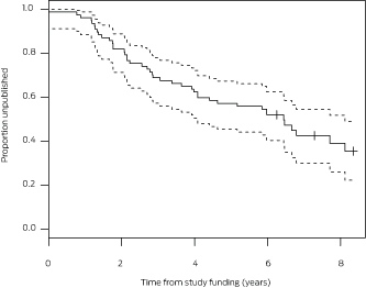
We can visualise survival over time using a Kaplan–Meier plot, which shows the proportion who have yet to develop dementia on the y axis against time on the x axis. The plot accounts for censoring, so the denominator declines as we move from left to right as more participants are censored or get dementia. We can plot separate survival lines for categorical predictors, so we could have lines for smokers and non-smokers and see if and when the lines begin to diverge.

An example of a Kaplan–Meier plot is provided in Box 2, which shows the time between receiving a National Health and Medical Research Council project grant for a clinical trial and the time to publishing the protocol.4 The x axis shows time in years and the y axis shows the proportion yet to publish. After 8 years, 0.39 (or 39%) of studies had not yet published a protocol paper (95% CI, 0.26–0.52). Another way to read the graph is to look at the point at which 50% of papers have been published; in this case, about 6 years (ie, median time to publication is 6 years). A log-rank test can be used to perform a test of equality between survival curves and obtain a P value, provided the survival curves do not cross.

We can also adjust for other potential predictors or confounders of survival using a Cox proportional hazards model.5 In our example, we would model the hazard of dementia, where the hazard is the probability that participants move from no diagnosis to having a diagnosis of dementia in the next short period of time; it can be thought of as the average risk of developing dementia at any instant in time. The Cox model estimates a general baseline hazard over time, and this general baseline hazard is then multiplied by a function of the predictors to give a hazard ratio (with 95% confidence intervals). In our example, we could set non-smokers as the reference group and look at the hazard ratio of dementia for smokers. If this ratio were greater than one, it would mean that smoking sped up the time to diagnosis (on average) compared with not smoking, and if it were less than one, then smoking slowed the progression. When reporting our results we should include the total follow-up time and the average follow-up time per participant.6

Extensions to survival analysis

Recurrent events

Although most studies only include time to first event, we could extend our example to include recurrent events for the same participant; for example, hospital admissions between smokers and non-smokers. Imagine a participant is recruited and is admitted to hospital at year 3. We would include a row in the data that had a time of 3 years and a censored value of false. We could include them again based on their readmission in year 7 by adding another row in the data with their second admission, new time of 4 years and a unique ID number (participant 5.1 and 5.2 in Box 1). This is useful because it makes the results more generalisable as we are not excluding valid data, and it increases our sample size without the additional logistical cost of obtaining consent from another participant. However, we do need to account for the dependence in the data from getting results from the same participant when dealing with recurring events.

Time-varying covariates

The Kaplan–Meier and Cox proportional hazards methods discussed above assume that the covariate groups (eg, smoker or non-smoker) are defined at the beginning of the study time and remain the same throughout. But how should we handle a participant who started out as a smoker but quit after 3 years? Methods exist to handle so-called time-varying (or time-dependent) covariates. The methods allow the first 3 years of follow-up to contribute to the smoking dataset and the remaining years to contribute to the non-smoking dataset. However, great care should be taken to make sure that this fits the biology being described; for example, a time-varying analysis would be suitable for an outcome such as myocardial infarction, where the risk is more closely determined by current status, but not suitable for cancer, where the risk is determined by cumulative long term exposure. In this case, one would have to code cumulative years of smoking in relation to cancer risk.

Immortal time bias

What if we decided to simply analyse smokers and non-smokers who survived at least to 65 years of age, when dementia can plausibly develop? Could we not just look at time to dementia within these groups? The flaw in this logic is that people must survive until age 65; this might selectively deplete the cohort of smokers who could have died from heart attacks, strokes, chronic obstructive pulmonary disease or cancers before then, and might skew the smokers who have made it to that point. Excluding these previous years from the analysis leads to what is called immortal time bias.7 Another example of this bias is when researchers study the impact of an event during a hospital stay (eg, a hospital-acquired infection) on length of stay. Many researchers simply compare the total lengths of stay for patients who did and did not experience an infection, but this includes the time before participants had an infection, which introduces immortal time bias.8,9 Another way to understand this is to think that the longer one is in hospital, the greater the risk of developing infection — a chicken and egg problem. Including this immortal time in the study design means the effect of infection on length of stay is greatly exaggerated.

Competing risk

Another important issue in survival analysis is competing risks which can produce counterintuitive results.10,11 To understand this, let’s return to our example where we follow smokers and non-smokers over time until the diagnosis of dementia. What if someone drops out at age 70 without having developed dementia? As we saw above, we can simply censor them so that we can use their data up to that point. But what if they dropped out because of death? Can we still censor them at that point? Technically, this would not be correct, because censoring assumes that the person is still at risk beyond this point but that they are simply not included in the dataset. Someone who drops out because of a competing risk such as death — that is, an event that means they can no longer experience the outcome — has to be treated differently. Otherwise, a group of smokers might show less dementia simply because they have more deaths from cardiovascular disease. A solution is to use separate survival analyses for every competing risk as well as the outcome of interest, to try to give a complete picture of the participants’ risks over time.

Truncation

Another important concept to understand in survival analysis is truncation, which occurs when some data are discarded because they fall before or after the study time period. In our example of smokers and non-smokers being followed for time to dementia diagnosis, it is possible that a person was given a diagnosis of dementia before their first visit to a GP and hence would not be included in the study; such a person would be “left” truncated, because this occurs on the left of the graph.12

Survival analyses are a highly useful statistical method that can help find predictors of risk and help infer causality because we examine exposures before outcomes. However, like any study design, survival analysis relies on accurate data and, because of the complexities caused by time, there is more potential for the data to be incomplete, leading to biased estimates of risk.

Box 1 – Hypothetical example of survival data that uses time compared with binary data that ignores time

Box 2 – Kaplan–Meier plot showing the time between receiving a National Health and Medical Research Council project grant for a clinical trial and the time to publishing the protocol*

---

* Dotted lines show 95% confidence intervals.

References

- Attia JR, Jones MP, Suthers B. Aiming for the truth: understanding the difference between validity and precision. Med J Aust 2016; 205: 392-394.
- Attia JR, Jones MP, Hure A. Deconfounding confounding part 1: traditional explanations. Med J Aust 2017; 206: 244-245.
- Attia JR, Oldmeadow C, Holliday EG, Jones MP. Deconfounding confounding part 2: using directed acyclic graphs (DAGs). Med J Aust 2017; 206: 480-483.
- Strand LB, Clarke P, Graves N, et al. Time to publication for publicly funded clinical trials in Australia: an observational study. BMJ Open 2017; 7: e012212.
- Kalbfleisch JD, Prentice RL. The statistical analysis of failure time data. 2nd ed. New York: John Wiley, 2011.
- von Elm E, Altman DG, Egger M, et al. Strengthening the reporting of observational studies in epidemiology (STROBE) statement: guidelines for reporting observational studies. BMJ 2007; 335: 806.
- Lévesque LE, Hanley JA, Kezouh A, Suissa S. Problem of immortal time bias in cohort studies: example using statins for preventing progression of diabetes. BMJ 2010; 340: b5087.
- Trentino KM, Swain SG, Burrows SA, et al. Measuring the incidence of hospital-acquired complications and their effect on length of stay using CHADx. Med J Aust 2013; 199: 543-547.
- Barnett AG, Beyersmann J, Allignol A, et al. The time-dependent bias and its effect on extra length of stay due to nosocomial infection. Value Health 2011; 14: 381-386.
- Andersen PK, Geskus RB, De witte T, Putter H. Competing risks in epidemiology: possibilities and pitfalls. Int J Epidemiol 2012; 41: 861-870.
- Wolkewitz M, Cooper BS, Bonten MJM, et al. Interpreting and comparing risks in the presence of competing events. BMJ 2014; 349: g5060.
- Klein JP, Moeshberger ML. Survival analysis: techniques for censored and truncated data. 2nd ed. Springer, 2003: pp 63-87.
Provenance: Commissioned; externally peer reviewed.
Interpreting Australian Stillbirth Rate Trends: Implications for Surveillance and Continuous Quality Improvement
Aleena M. Wojcieszek, Kirstine Sketcher-Baker, Christine Andrews, Michael Coory, Imogen Kettle, Melissa Malivoire, David Ellwood, Vicki Flenady
Paracetamol in Pregnancy: Uncertain Evidence, Certain Consequences
David J. Tunnicliffe, Miranda Cumpston, Debra Kennedy, Margie Danchin, Armando Teixeira-Pinto
Fatty Liver Disease in Australia: A Narrative Review on the Epidemiology, Natural History, Prognostication and Management in People With Metabolic Dysfunction
Karl Vaz, Daniel Clayton-Chubb, William W. Kemp, Stuart K. Roberts, Ammar Majeed
Birth prevalence, clinical sequelae, and management of congenital cytomegalovirus infections in Australia, 1999–2023: a national prospective study
Ece Egilmezer, Suzy M Teutsch, Carlos Nunez, Stuart T Hamilton, Adam W Bartlett, Pamela Palasanthiran, Elizabeth J Elliott, William D Rawlinson
The number of cancer‐related deaths that could be attributable to spatial disparities in survival in Australia, 2010–2019: a retrospective population‐based cohort study
Charlotte K Bainomugisa, Jessica Cameron, Paramita Dasgupta, Peter Baade
Mandatory research projects during medical specialist training in Australia and New Zealand
Paulina Stehlik, Caitlin Brandenburg, David A Henry