Deconfounding confounding part 3: controlling for confounding in statistical analyses

The traditional concept of confounding was previously introduced in this Key Research Skills series — a confounder is a variable that is associated with both the exposure and outcome of interest without being an intermediate on the causal pathway between them.1 Although the earlier article also outlined how a randomised controlled trial (RCT) can be used as a solution to handle confounding at the study design phase, it is not always feasible to use an RCT. For example, consider a study looking at the association between smoking (exposure) and cardiovascular disease (CVD; outcome). It is not ethical to randomly assign people to smoke! The alternative is to conduct an observational study in which confounders are carefully identified, measured without too much error, and adjusted for in the statistical analysis.

Why is confounding important and what can be done about it?

Confounding is one of the most important issues in establishing causality in medical research, and probably the most important cause of spurious associations in observational epidemiology.2 Health consequences of flawed research findings can be serious, as evidenced by the case of hormone replacement therapy, which looked so promising in multiple studies that did not control for confounding by socio‐economic status, but was completely reversed in the Women's Health Initiative trial, which controlled for socio‐economic status.3,4 Unless controlled for, confounding distorts the estimate of the exposure–outcome association and makes it difficult to measure the true association.

A common way to quantify the magnitude of confounding is based on a rule of thumb,5 namely that if a parameter estimate changes by more than 10% when an additional variable is added to a model, then this variable is considered to be a potentially strong confounder; the place of this variable in the causal pathway needs separate consideration. A wider range of approaches to quantifying confounding has been explored,6 and causal pathways appear in earlier articles in this series.7,8

Methods to control for confounding in the study design phase include randomisation (to ensure participants have an equal chance of being in any arm of the RCT, so that the distribution of confounders in arms are similar), matching (eg, age, sex, smoking status in case–control studies, especially when the outcome is rare) and restriction (restricting the study to a particular level of the confounder variable). However, controlling for confounding in the study design phase is not always feasible. For example, some research questions do not permit random assignment of participants. Similarly, when there are multiple confounders to be controlled for, a matched study can become unwieldy. Restriction of a study to individuals with the same levels of the confounding factors may affect sample size and generalisability, and limit the scope of the study.

This article focuses on controlling for confounders in the analysis phase. Stratification, statistical adjustment (including but not restricted to methods such as ANCOVA [analysis of covariance]) and standardisation are fundamental methods that can be used to control for measured confounding variables.

Controlling for confounding using stratification

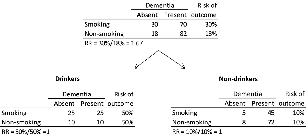
Stratification involves splitting the study sample into subsamples based on categories of the confounding variable and looking at the exposure–outcome relationship separately within categories. Attia and colleagues1 use the example of the smoking (exposure) and dementia (outcome) relationship where alcohol consumption is postulated to be a confounder. While the risk of developing dementia was 67% higher among smokers versus non‐smokers in the whole sample (crude relative risk [RR], 1.67), stratification by alcohol consumption showed that the effect of smoking was completely confounded by alcohol consumption (Box 1); elevated smoking–dementia risks were not observed in drinkers or non‐drinkers (RR, 1 in both groups).

Stratification can be used to evaluate potential confounders.9 If stratum‐specific estimates are similar (as in this case, an RR of 1 in both drinkers and non‐drinkers) but are different to the crude estimate (RR, 1.67), the interest lies in combining the stratum‐specific estimates rather than reporting them separately. Stratum‐specific estimates can be combined using the Cochran–Mantel–Haenszel method, which weights the association between two binary variables at different levels of a confounding variable by the number of observations at each level.9 The test statistic can be thought of a pooled statistic over all the strata (levels of confounder variable), weighted by the number of observations in each stratum. In this case, the RR_cmh is 1. If stratum‐specific estimates are different, then the relationship between exposure and outcome is different in each stratum, indicating effect modification; instead of combining stratum‐specific estimates, they need to be reported separately. Stratification may involve splitting data into more than two categories (eg, 0, 1–14 and > 14 alcoholic drinks per week).

While stratification is intuitive and easy to use, it cannot be used to control for multiple confounding variables at the same time. Further, it cannot be used to control for continuous variables such as age, which is usually a strong confounder for many exposure–outcome relationships in epidemiology. Residual confounding can also occur whenever a continuous variable has artificial thresholds imposed, such as categorising age or dichotomising a response at the median.

Controlling for confounding using standardisation

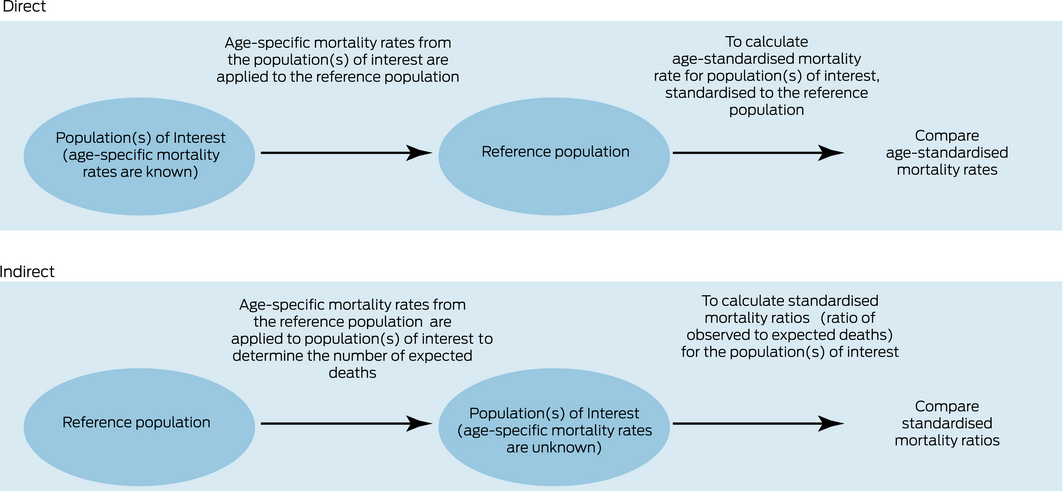
A second approach to controlling for confounding is through the presentation of standardised estimates or rates. These allow the researcher to compare patterns across subgroups in the population. A reference group is chosen and the distribution of key characteristics such as age and sex is weighted in the other groups to match the reference group. Death rates and disease incidence are usually strongly related to age and often differ for the two sexes. It is important to allow for the age–sex distribution of the population, particularly when comparing rates over periods of time where the population distribution has changed. This can be done by either direct or indirect standardisation.

For example, to age‐standardise using the direct method, a reference population is chosen and rates of the disease in the standard population are calculated applying age‐specific rates from each population of interest. An age‐standardised rate is a weighted average of the rates in the different age groups. Indirect age‐standardisation can be used if we do not have age‐specific rates for the population of interest, but do have the age structure of the populations of interest and age‐specific rates in a standard population. Rates in the standard population are applied to the populations of interest to determine the number of expected events. Box 2 demonstrates the workflows for the standardisation methods. In the study presented in Box 3,10 the rates of acute myocardial infarction (AMI) per 1000 person‐years have been included, age‐standardised and sex‐standardised (where applicable) to the 2006 New South Wales population, in 5‐year age groups, using the direct method. Although the age and sex distributions may differ by smoking categories and crude rates may not be meaningful for comparison, the age‐ and sex‐adjusted rates can be compared. There is a nearly threefold increase in the age‐ and sex‐standardised rate of AMI in current smokers compared with never smokers (6.20 per 1000 person‐years v 2.84 per 1000 person‐years).

Controlling for confounding using statistical adjustment

Statistical adjustment involves including confounding variables in the regression model when modelling the exposure–outcome relationship. For instance, consider the study results presented in Box 3,10 which look at the risk of developing AMI in relation to smoking. Confounders identified a priori include age, sex, region of residence, alcohol consumption, income and education. Multiple confounders are adjusted for simultaneously in Cox regression models. Compared with never smokers, current smokers are 2.45 times more likely to develop AMI after controlling for confounders (ie, holding them fixed at their reference level). Note that the focus here is not on the effect of confounding but on controlling for it. Sex is associated with both smoking and AMI, but is not on the causal pathway in the smoking–AMI relationship (ie, it meets the criteria for a confounder) and the overall analysis is adjusted for sex. However, estimates are also presented separately for men and women (stratified by sex) since the smoking and CVD relationship was different in men and women, as indicated by the significant interaction by sex. Compared with never smokers, smokers are 2.26 times more likely to develop AMI among men; the corresponding risk among women is 2.87 times. Note that the focus here is on the effect of confounding; that is, stratum‐specific estimates. Body mass index (BMI) was considered likely to contribute, at least partially, to the causal pathway between smoking and CVD and does not fully meet the criteria for a confounder. Instead of adjusting for BMI, hazard ratios derived from Cox models were estimated within subgroups of BMI. A further refinement that is possible with adjusted models is that effect modification can also be examined using interaction terms, which are product variables in the regression model that represent an interaction between two predictor variables.

A regression model estimates the effect of the exposure of interest on the outcome, adjusting for confounders. An interaction term allows quantification of change to this effect estimate when it occurs in combination with a third variable or confounder. The interpretation of interaction terms is dependent upon whether they appear in an additive model, such as a linear regression, or a multiplicative model, such as a logistic regression model on the logit scale. For example, in a linear regression model of age, sex and BMI on physical activity outcomes for patients with kidney disease,11 the interaction between age and haemodialysis is expressly listed as an effect in the linear regression model. For every extra year of age, the predicted level of physical activity drops by an extra 1675.8 units for haemodialysis patients compared with control subjects. In the CVD study discussed above,10 there is significant interaction by age group in the relationship between smoking and CVD. The interpretation is handled by reporting the P value for the interaction term, and then reporting parameter estimates (hazard ratios) separately for age groups. This means that the specific parameter estimates for the interaction terms are not presented. For more information, a broad ranging tutorial on interactions in non‐linear models is available.12

Conclusion

Introductory textbooks9 commonly refer to stratification as a useful method to control for confounding, which it is, but it is not commonly used in practice owing to its limitations. Similarly, standardisation is often proposed as a helpful method of presenting results, but it also has limitations in terms of the number of variables that can be controlled for. Although control for confounding using statistical adjustment is relatively easier during the analysis phase, one needs to think carefully about causal pathways and potential confounders during the study design phase itself. Clinical knowledge is needed to identify potential confounders which are not on the causal pathway between the exposure and the outcome — no statistical test can verify this assumption. Further, we can control for confounding in the analysis phase only if we have measured the confounder. Depending on the research question and the intended readership of the research, one may choose to control for confounding or describe modification of effect estimates.

Box 1 – Stratification by alcohol consumption

---

RR = relative risk.

Box 2 – Workflows for the direct and indirect standardisation methods

---

References

- Attia JR, Jones MP, Hure A. Deconfounding confounding part 1: traditional explanations. Med J Aust 2017; 206: 244–245. https://www.mja.com.au/journal/2017/206/6/deconfounding-confounding-part-1-traditional-explanations
- Von Elm E, Egger M. The scandal of poor epidemiological research. BMJ 2004; 329: 868.
- Manson JE et al. The Women's Health Initiative hormone therapy trials: update and overview of health outcomes during the intervention and post‐stopping phases. JAMA 2013; 310: 1353–1368.
- Petitti D. Commentary: hormone replacement therapy and coronary heart disease: four lessons. Int J Epidemiol 2004; 33: 461–463.
- Lee PH. Is a cutoff of 10% appropriate for the change‐in-estimate criterion of confounder identification? J Epidemiol 2014; 24: 161–167.
- Vanderweele TJ. Principles of confounder selection. Eur J Epidemiol 2019; 34: 211–219.
- Attia JR, Oldmeadow C, Holliday EG, Jones MP. Deconfounding confounding part 2: using directed acyclic graphs (DAGs). Med J Aust 2017; 206: 480–483. https://www.mja.com.au/journal/2017/206/11/deconfounding-confounding-part-2-using-directed-acyclic-graphs-dags
- Jones MP, Walker MM, Attia JR. Understanding statistical principles in correlation, causation and moderation in human disease. Med J Aust 2017; 207: 104–107. https://www.mja.com.au/journal/2017/207/3/understanding-statistical-principles-correlation-causation-and-moderation-human
- Webb P, Bain C, Page A. Essential epidemiology 3rd ed. Cambridge: Cambridge University Press, 2017.
- Banks E, Joshy G, Korda RJ, et al. Tobacco smoking and risk of 36 cardiovascular disease sybtypes: fatal and non‐fatal outcomes in a large prospective Australian study. BMC Med 2019; 17: 128.
- Johansen KL, Chertow GM, Ng AV, et al. Physical activity levels in patients on haemodialysis and health sedentary controls. Kidney Int 2000; 57: 2564–2570.
- Karaca‐Mandic P, Norton EC, Dowd B. Interaction terms in nonlinear models. Health Serv Res 2012; 47: 255–274.
Provenance: Commissioned; externally peer reviewed.
Driving Implementation-Focused Change for Gender Equity in Medical Leadership: A Consensus-Based Priority-Setting Approach
Belinda Garth, Jenny Proimos, Thuy Vy Nguyen, Sally Cross, Sarah Whitelaw, Helena J. Teede
Advancing Gender Equality in Australian Healthcare Leadership: Why National Targets Matter and What It Means for Healthcare Employers
Belinda Garth, Nicole Pope, Jenny Proimos, Helena J. Teede
Centring Aboriginal and Torres Strait Islander Voices: A Framework for Culturally Safe and Racism-Free Healthcare
Elissa Elvidge, Roianne West, Karen Nicholls, Kiara Harvey, Yeena Thompson, Geraint B. Rogers, Yin Paradies
Medical Colleges Have an Obligation to Ensure Full Participation in Clinical Quality Registries
Robert J. Aitken, Julian A. Smith, Guy J. Maddern