Understanding statistical principles in linear and logistic regression

A previous article in this series assessed the association between two variables.1 Here, we introduce the concept of multivariable regression.2-4 A regression model establishes the relationship between one or more exposure, or explanatory, variables (such as height, weight and sex) and an outcome (such as body mass index or smoking status). The resulting model describes the nature of the relationship between explanatory variables and outcome, and can be used to predict an unknown outcome value based on given values of the explanatory variables. The term “multivariate” indicates more than one outcome being analysed concurrently, and “multivariable” indicates more than one explanatory variable being analysed. This article concentrates on one outcome and multiple explanatory variables.

Previously in this series, Jones and colleagues examined the relationship in hypothetical data between gastrointestinal symptom rating scale (GSRS) score and mast cell count.1 We use the same dataset to demonstrate how regression models work, without reference to causal pathways.

Linear regression models

The simple linear regression model is the best-fitting straight line between a continuous outcome and an explanatory variable. Consider the plot of GSRS score versus mast cell count in Box 1. The points represent the data values, the bold line represents the fitted regression line and the dashed lines represent the vertical distances between the actual values of the outcome and those fitted by the regression line. These vertical distances are also called “residuals” or “errors”. The line of best fit is the one which is closest to the data points (ie, that minimises the residuals). A regression model is a reasonable model here as the model assumptions are satisfied: the spread of errors about the line remains constant for the entire length of the line, normal distribution of errors, and a linear relationship between continuous explanatory and outcome variables.5 Because some of these residuals are positive and others are negative, the squares of the residuals, rather than the actual residuals, are minimised. This is why linear regression is sometimes referred to as least squares regression. Least squares regression is the typical mathematical method for determining the line of best fit, and is generally undertaken using a statistical software package.

Box 2 shows the results of a simple linear regression as typically reported by journals. The results include estimates of the regression parameters (also called coefficients), 95% confidence intervals, and the t statistic and P value from a hypothesis test which indicates whether there is a statistically significant relationship between the explanatory variable and the outcome. The parameter estimates describe the relationship between the explanatory variable and the outcome. The value for mast cell count is 0.096, which means that for every unit increase in mast cell count, the GSRS score is estimated to rise by 0.096 (95% CI, 0.088–0.103). The P value is < 0.001, indicating a statistically significant result; that is, there is strong evidence of a non-zero parameter relating mast cell count to GSRS score in the population.

The R² value is a number between 0 and 1 that describes how well the model fits the data — the higher the better. In Box 2, the R² value for the simple linear regression model is 0.76. A low R² value may indicate that important explanatory variables have been excluded from the model. The R² value is a broadly useful measure of how good the model is; however, it has a couple of pitfalls. Its validity depends on model assumptions being correct, and its value increases as the number of explanatory variables increases, even if these are not related to the outcome. The R² value can be adjusted to combat this increase, and in Box 2 we see that the adjusted R² value remains at 0.76 even though a second variable has been included in the model.

Often we need to consider additional variables other than the explanatory variable of interest and the outcome; to control for confounding,6,7 where the effect of the explanatory variable of interest (eg, GSRS score) is mixed up with the effect of some other variable (eg, sex), or to increase precision of coefficient estimates (less variability in the outcome if we control for other variables). Multiple linear regression models include more than one (and sometimes many) explanatory variables. The advantage of these models is that multiple variables can be considered at the same time. When additional variables are included in the model, we estimate the association between the explanatory variable of interest and the outcome, holding the additional variables constant. This provides a way of adjusting for (or accounting for) the additional variables included in the model. Box 2 shows the results for multiple linear regression where the effect of mast cell count is adjusted for sex. For each unit increase in mast cell count, the GSRS score is estimated to increase by 0.096 (95% CI, 0.088–0.104), adjusted for sex. The GSRS score is estimated to be 0.22 higher for females relative to males (95% CI, − 1.009 to − 1.444), adjusted for mast cell count. The relationship between mast cell count and GSRS score is significant (P < 0.001) and the relationship between sex and GSRS score is not statistically significant (P = 0.726).

Logistic regression

If the outcome variable is binary, the assumptions for linear regression described above are not met. The usual method of regression analysis for binary outcomes is logistic regression and, as with linear regression, either a single (simple) or many (multiple) continuous or categorical explanatory variables can be included.8 Binary logistic regression can also be extended to categorical outcomes with more than two categories (multinomial) or ordered categories (ordinal).

Logistic regression basically involves moving from modelling the relationship between explanatory variables and a continuous outcome, to modelling the relationship between explanatory variables and the log odds of a binary outcome (a logistic transformation of the outcome), hence the name. Least squares regression is no longer used to estimate the parameters; maximum likelihood is the algorithm employed.

Returning to our hypothetical data, we have a binary outcome variable “presence of gastrointestinal (GI) symptoms” with values “Yes” and “No”. Interest centres on modelling the effect of mast cell count and sex on the probability of GI symptoms.

The scatter plot in Box 3 shows that with a binary outcome such as GI symptoms, there is little sense in fitting a straight line between the two outcomes. The box plots suggest a relationship between mast cell count and presence of GI symptoms. A logistic regression model not only provides a numerical measure of the size of the association but can also include adjustment for confounding variables such as sex.

Box 4 shows the results of the multiple logistic regression in typical journal format. The relationship between explanatory variables is expressed in terms of odds ratios. These are not the same as risk ratios, although when the outcome is rare they are often about equal. However, for common outcomes, odds ratios are more extreme than relative risks.

The correct interpretation of the odds ratio is that the odds of having GI symptoms are estimated to be 1.04 times higher (95% CI, 1.03–1.05) for every one unit increase in mast cell count, adjusted for sex. The odds of GI symptoms are estimated to be 1.03 times higher (95% CI, 0.45–2.36) for females, adjusted for mast cell count. The narrower confidence interval for mast cells, compared with sex, reflects not only the precision of the estimate but also the measurement scale; a one unit increase in mast cell count is very small. The relationship between mast cell count and the presence of a high GSRS score is statistically significant (P < 0.001), but the effect of sex on the presence of a high GSRS score is not (P = 0.942).

There is no statistic analogous to the R² value for logistic regression. Some packages report measures such as a pseudo-R² value, but these are of low validity. One of many formal tests is the Hosmer–Lemeshow test,8 where a high P value indicates a better fit. The P value for the goodness-of-fit test (Box 4) is 0.36, indicating that the model is a reasonable fit to the data. A poor fit may indicate the exclusion of important explanatory variables. However, this test is dependent on user-selected groups and, depending on your data, other tests may be more appropriate. Similar to the requirement for a linear association between a continuous explanatory variable and outcome for linear regression, an important assumption for logistic regression is that there is a linear relationship between a continuous variable and the log odds of the outcome. A significant lack of fit may indicate a violation of assumptions, and other models may fit better.

Conclusion

Both linear and logistic regression belong to the family of generalised linear models, which model the relationship between explanatory variables and a large range of different types of outcomes. We have provided a brief overview of linear and logistic regression for modelling the relationship between one or more explanatory variables and an outcome (either continuous or categorical). It is important to remember that different types of models are required for different types of outcomes, and that assumptions, interpretations of model parameters and measures of overall fit will vary for different types of models.

Box 1 – Scatter plot showing the data points and fitted linear regression line for the association between gastrointestinal symptom rating scale (GSRS) score and mast cell count

---

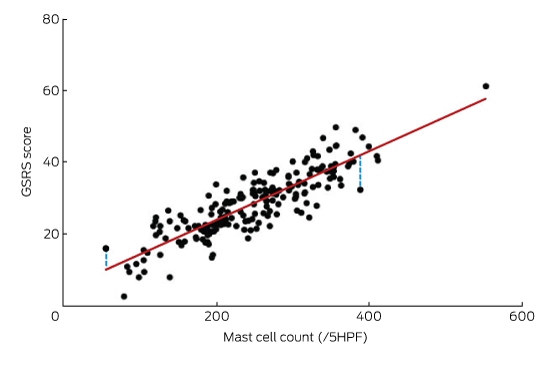
HPF = high power field.

Box 3 – Scatter plot and box plot of high gastrointestinal (GI) symptom rating scale score (0 = absent, 1 = present) by mast cell count

---

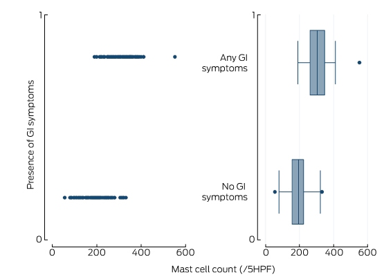
HPF = high power field.

References

- Jones MP, Walker MM, Attia JR. Understanding statistical principles in correlation, causation and moderation in human disease. Med J Aust 2017; 207: 104-106.
- Altman DG. Practical statistics for medical research. London: Chapman & Hall/CRC, 2006.
- Armitage P, Berry G, Matthews JNS. Statistical methods in medical research. 4th ed. Malden, MA: Blackwell Science, 2002.
- Clayton D, Hills M. Statistical models in epidemiology. Oxford: Oxford University Press, 1993.
- Kirkwood BR, Sterne JAC. Essential medical statistics. Malden, MA: Blackwell Science, 2003.
- Attia JR, Jones MP, Hure A. Deconfounding confounding part 1: traditional explanations. Med J Aust 2017; 206: 244-245.
- Attia JR, Oldmeadow C, Holliday EG, Jones MP. Deconfounding confounding part 2: using directed acyclic graphs (DAGs). Med J Aust 2017; 206: 480-483.
- Hosmer DW, Lemeshow S. Applied logistic regression. 2nd ed. New York: Wiley, 2000.
Provenance: Commissioned; externally peer reviewed.
Interpreting Australian Stillbirth Rate Trends: Implications for Surveillance and Continuous Quality Improvement
Aleena M. Wojcieszek, Kirstine Sketcher-Baker, Christine Andrews, Michael Coory, Imogen Kettle, Melissa Malivoire, David Ellwood, Vicki Flenady
Paracetamol in Pregnancy: Uncertain Evidence, Certain Consequences
David J. Tunnicliffe, Miranda Cumpston, Debra Kennedy, Margie Danchin, Armando Teixeira-Pinto
Fatty Liver Disease in Australia: A Narrative Review on the Epidemiology, Natural History, Prognostication and Management in People With Metabolic Dysfunction
Karl Vaz, Daniel Clayton-Chubb, William W. Kemp, Stuart K. Roberts, Ammar Majeed
Birth prevalence, clinical sequelae, and management of congenital cytomegalovirus infections in Australia, 1999–2023: a national prospective study
Ece Egilmezer, Suzy M Teutsch, Carlos Nunez, Stuart T Hamilton, Adam W Bartlett, Pamela Palasanthiran, Elizabeth J Elliott, William D Rawlinson
The number of cancer‐related deaths that could be attributable to spatial disparities in survival in Australia, 2010–2019: a retrospective population‐based cohort study
Charlotte K Bainomugisa, Jessica Cameron, Paramita Dasgupta, Peter Baade
Mandatory research projects during medical specialist training in Australia and New Zealand
Paulina Stehlik, Caitlin Brandenburg, David A Henry