Sampling: how you choose people is as important as how you analyse their data

Much attention is paid in research publications to the methods of statistical analysis. Research design, in contrast, receives less consideration, despite the fact that it is critical; if the research design is poor, no amount of complex statistical analysis can extract useful information from the data collected. In this article, we focus on the selection of subjects for medical research studies, and outline several sampling strategies and their implications for statistical analysis. As a high level overview of sampling in medical research, we do not go into deep technical detail. Further, we discuss how to obtain a sample, but not how large the sample should be; we refer readers to Lachin1 for an introduction to the important topic of sample size and statistical power calculations.

What are sampling schemes?

A sampling scheme is the process used by researchers to select the individuals about whom they will collect data for testing a hypothesis or answering a research question. The individuals may be patients in a clinic, members of a special group (eg, twins), or part of the general population. The word “sampling” is, however, critical: with very few exceptions (such as the Australian census), data are collected for only a sample of individuals, but the investigator wants to make inferences about the population from which the sample was drawn. For example, we might conduct a public health survey to estimate the prevalence of type 2 diabetes in the Australian population, collecting data from a sample of 500 people (n = 500). We establish whether each of these individuals has type 2 diabetes, and may find that 60 have the disorder, yielding a sample prevalence of 12%. Our real question, however, is whether the sample is representative of the Australian population; ie, whether the population prevalence of type 2 diabetes is also 12%. It is therefore critically important that we select a sample which faithfully represents the population of interest if our sample is not to produce misleading results.

Statistical adjustments for bias

We will discuss how oversampling, cluster sampling and convenience sampling are all likely to produce samples that differ from the populations we wish to understand in features that are important to our investigation. This is a form of bias, and any conclusions we draw from statistical analysis of the sample may be misleading. We say “may” because, if we can quantify the source of bias, we can correct for it in the statistical analysis. Indeed, a range of statistical methods have been developed to cope with sampling schemes that yield samples not closely representative of the population of interest.

Common sampling designs

Simple random sampling (SRS)

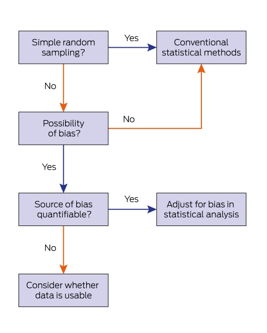
This is the workhorse of many areas of medical research, particularly in public health and epidemiology. If SRS is applied strictly, every member of a target population has an equal chance of being selected in the sample,2,3 and SRS will therefore produce a sample with representation from across the spectrum of this population. SRS is depicted in Box 1(a), where the red dots represent individuals drawn randomly from the population. The key term in SRS is “random”; if the selection is genuinely random, it is extremely unlikely that our sample will be dominated by any particular subgroup from the population, and it should therefore be broadly representative. In practice, truly random sampling is not always possible without resources that are beyond the capacity of many researchers. Not all non-random samples are biased, but SRS reduces the risk of bias. When a sample is obtained by non-random sampling, there is greater onus on the researcher to ensure that the sample is not biased relative to the sampled population; if it is not, statistical analysis can proceed as though SRS had been employed (Box 2).

Stratified random sampling

SRS works well in many areas of medical research, but not in all areas of public health. For example, a population may include small but important subgroups that, because of their size, may by chance be completely omitted from a relatively small sample. In these cases, we might stratify the population to ensure that we recruit a reasonable number of individuals from even the smallest stratum.2 In doing so, we can recruit the same fraction of members from each stratum — as in Box 1(b), where we recruit one-third of each stratum — or recruit proportionately more members from smaller than from larger strata (“oversampling”)3 — as in Box 1(c), where we sample one-half of the smaller stratum, but one-third of the larger. As some groups are deliberately over-represented, oversampling produces a non-representative sample. When analysing such a sample, over-representation must be compensated by weighting individuals according to the proportional size of the stratum from which they were drawn.

Adjusting for oversampling

Let us take the simplest of statistics, the sample mean:∑i=1nxin

The problem with applying this formula after oversampling is that the contribution of the oversampled group to n is over-represented relative to the population. However, we can adjust the formula so that the weight of an individual in the analysis is inversely proportional to the extent to which their stratum was oversampled.3 This correction is possible because we understand and can quantify the source of the difference between the population and sample characteristics (Box 2).

Cluster sampling

Another convenient approach to sampling is to recruit a number of groups, such as patients of general practices or hospital clinics, and to then sample from each group. This is known as cluster sampling2,3 because clusters are randomly sampled (general practices, clinics, etc.) before all or a random sample of members of each cluster is recruited. In Box 1(d), the oval shapes represent clusters and the non-blue dots are the sampled members of that cluster. To avoid producing an irretrievably unrepresentative sample, the clusters must provide a broad coverage of the population. If, for example, the clusters were dominated by elderly patients or more seriously ill patients, the entire sample will be unrepresentative, and, unlike probability sampling, there is no way to compensate for this in the statistical analysis.

Adjusting for cluster sampling

A second key feature of cluster random samples is that the features of members are more likely to be correlated within a cluster than with those of other clusters. Cluster sampling is thus likely to violate the usual assumption of independence of observations, and to therefore overcount the effective sample size; this will lead in turn to underestimating standard errors (and P values). Consequently, any statistical analysis of clustered random samples must use methods applicable to correlated data.3

One approach to measuring similarity within clusters is to calculate the intraclass correlation (ICC).4 Leslie Kish defined “design effect” as 1 + δ (n − 1), where δ is the ICC.5 As the design effect estimates the ratio of the actual sample variance to the variance assuming SRS, it can be used to estimate what the sample size would have been in an SRS model (the effective sample size), and corrected standard errors and P values can be calculated. This approach may also be applied in multistage (complex) sampling.

Multistage (complex) random sampling

Complex or multistage sampling designs are also often used for practical convenience. Collecting a national population sample could involve sending research staff to numerous small towns, clinics or general practices across the country. Given the size of Australia and the logistics of obtaining agreement, it would be more practical to randomly sample a smaller number of towns/clinics/practices than to sample every member of the study population. As not every member of the population has the same probability of being sampled, this will not produce a simple random sample. As with cluster sampling, it is also likely that members of a sampling unit will resemble each other more than members of other units.6

Adjusting for complex sampling

There are a number of approaches to adjusting the statistical analysis of complex sampled data, but we do not have the space to discuss them all here. One approach is to view complex sampling as a special case of cluster sampling, as the sampling units can effectively be the same as sampling clusters.

Convenience sampling

Convenience samples are often used in many areas of medical research. Convenience samples are attractive to the researcher when obtaining a random sample is logistically difficult because of the cost of sampling from a broad geographic area or cultural barriers that hamper access to certain groups. These samples generally comprise individuals to whom the researchers have easy access, such as patients visiting an outpatient clinic, patients consulting a general practitioner, or people on a mailing list. The cost of convenience, however, is that the sample may not be representative of the population of interest,7 as shown in Box 1(e). For example, patients who consult a particular GP are likely to reside in a particular geographic area, with social and economic characteristics that are not representative of the general Australian population.

Adjusting for convenience sampling

We could view convenience sampling as an extreme form of oversampling, of groups that happen to be accessible. A fundamental problem, however, is that we have not sampled a known fraction of any stratum; indeed, we may not have well defined strata to sample. We have instead a sample that we strongly suspect is not representative of the population, but we have no way of statistically adjusting for this bias. The only potentially useful way of circumventing this problem is to re-define the population about which we can make inferences. For instance, if we had sampled from three outpatient clinics in Sydney teaching hospitals, we could make inferences about such outpatient clinics with some confidence. It would remain to be determined, however, whether it was useful to report on this population.

Summary of sampling schemes

Different sampling schemes produce samples that can offer very different views of the overall population; as indicated by the upper portions of Box 1, however, some will be representative of the population, others will not.

Does it really matter in practice?

Yes, it does! Ranmuthugala and colleagues,8 for example, sought to estimate the prevalence of elevated blood lead levels in children in central Sydney, an area in which exposure to lead was believed to be high. The authors applied two different sampling schemes, SRS and convenience sampling; the latter yielded a prevalence half that of stratified random sampling (5% v 10%; see the authors' table8).

Conclusion

While statistical analyses are simpler when SRS is applied, the good news is that not all sampling schemes that yield non-representative samples are problematic. Deliberate, well understood differences between sample and population characteristics can have practical advantages, and such biases can be corrected by adjusting the statistical analysis (Box 2). The real problem is when the bias in our sampling scheme cannot be quantified.

Our overview has dealt primarily with examples from health surveys and related research. The principles we have discussed can be applied broadly, but readers should be aware that other fields of medical research, such as genetic epidemiology9 and case–control studies,10 have specific sampling problems that need to be acknowledged.

Box 1 – The effect of the choice of sampling scheme on samples drawn from the same population

---

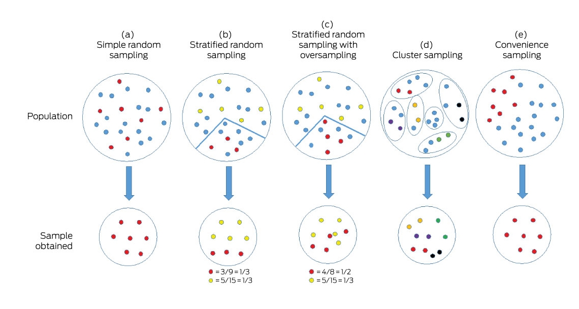
Dots in the population circle (upper section) represent individuals in the population; dots that are close together are individuals with similar traits. Non-blue dots in the population circle represent individuals selected in the sample (lower section). The samples resulting from simple random sampling (a) and convenience sampling (e) are superficially similar, but the sample in (a) is drawn from across the population while that in (e) is drawn from a subpopulation. The difference in samples yielded by schemes (b), (c) and (d) can be reconciled with (a) because the source of the difference is understood and can be quantified. For (e), however, the possible consequences of the sampling scheme must be discussed before proceeding to statistical analysis.

Box 2 – Decision tree linking the sampling scheme to the approach to statistical analysis

References

- Lachin JM. Introduction to sample size determination and power analysis for clinical trials. Control Clin Trials 1981; 2: 93-113.
- Kish L. Survey sampling. New York: John Wiley & Sons, 1965.
- Korn EL, Graubard BI. Analysis of health surveys. New York: John Wiley & Sons, 1999.
- Kish L, Frankel MR. Inference from complex samples. J R Stat Soc Series B 1974; 36: 1-37.
- Gulliford MC, Ukoumunne OC, Chinn S. Components of variance and intraclass correlations for the design of community-based surveys and intervention studies: data from the Health Survey for England 1994. Am J Epidemiol 1999; 149: 876-883.
- Osborne JW. Best practices in using large, complex samples: the importance of using appropriate weights and design effect compensation. Prac Assess Res Eval 2011; 16: 1-7.
- Hedt BL, Pagano M. Health indicators: eliminating bias from convenience sampling estimators. Stat Med 2011; 30: 560-568.
- Ranmuthugala G, Karr M, Mira M, et al. Opportunistic sampling from early childhood centres: a substitute for random sampling to determine lead and iron status of pre-school children? Aust N Z J Public Health 1998; 22: 512-514.
- Whittemore AS, Halpern J. Multi-stage sampling in genetic epidemiology. Stat Med 1997; 16: 153-167.
- Hu W, Cai J, Zeng D. Sample size/power calculation for stratified case-cohort design. Stat Med 2014; 33: 3973-3985.
Provenance: Commissioned; externally peer reviewed.
Driving Implementation-Focused Change for Gender Equity in Medical Leadership: A Consensus-Based Priority-Setting Approach
Belinda Garth, Jenny Proimos, Thuy Vy Nguyen, Sally Cross, Sarah Whitelaw, Helena J. Teede
The GenV Biobank: Enabling Biological Research in a Large Longitudinal Population-Representative Cohort of Australian Newborns and Their Parents
Katherine Lange, Kim L. Powell, Yeukai Mangwiro, Tony Frugier, Donna T. Geddes, Melissa Wake, Richard Saffery
A Match Made in Health Care: Can Ethics and Governance Better Support Impactful Implementation Research?
Natalie Taylor, Zhicheng Li, Cathelijne van Kemenade, Jackie Curtis, Patrick Bolton
Deconfounding confounding part 1: traditional explanations
John R Attia, Michael P Jones, Alexis Hure