Distributions and what to do when they are non-normal

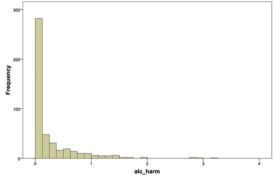
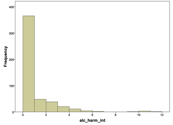
Medical researchers often want to find out how medically relevant outcomes are related to other factors. To do so, they carry out analyses and fit models that are based on assumptions about the nature of the research data. This article describes three methods which may be used when one commonly made assumption is not met. The methods are demonstrated on a real dataset in which the outcome is an index of harmful use of alcohol, with higher scores indicating a higher incidence of harmful behaviours. The frequency distribution of the outcome, alc_harm, is shown in Box 1.

The data were collected in an online survey (personal communication, Babucarr Sowe, 2016). The relationship of five of Sowe’s other measures to the harmful use of alcohol is examined in the analyses described here. These independent variables are age, sex, anxiety, drugs and religion (see the glossary in the Appendix). The Appendix also provides further information about the dataset.

Ordinary least squares (OLS) multiple regression analysis1 seeks to predict the values of an outcome variable with a linear model in which variables (or binary indicator variables representing categorical variables2) are weighted according to their contribution to predicting the outcome in the context of the other variables. Such diagnostic and prognostic models are commonly used in clinical practice.

The assumption of normality

If the association between the independent variables and the outcome is strongly linear, the differences between the actual and predicted values — the residuals — are small. Further, if the residuals are normally distributed, a key assumption underlying the use of tests of statistical significance in the regression analysis is met.

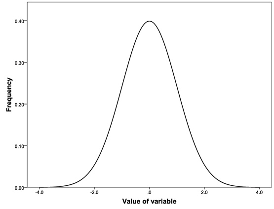
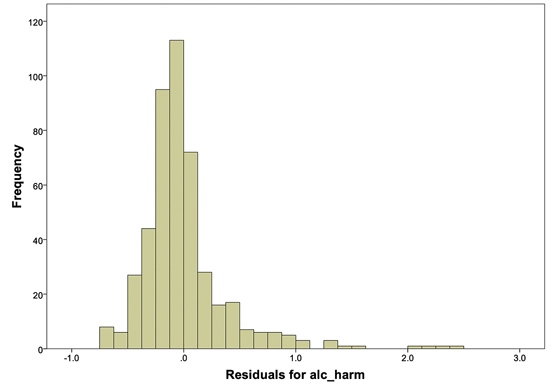
The theoretical normal distribution is defined by an equation that includes its mean and standard deviation. For our purposes, it is enough to note that the distribution is symmetrical and bell shaped, as shown in Box 2. The distribution of the residuals obtained from the regression of alc_harm on the independent variables, shown in Box 3, is non-normal (positively skewed). This result illustrates the problem addressed in the present article.

Dealing with non-normality

Because data obtained in clinical trials and surveys are seldom normally distributed, researchers have developed strategies to reduce the threat of departures from normality to the validity of statistical tests and the conclusions based on them.

One approach is to use non-parametric tests,3 which make no assumptions about the distribution of the outcome variable. Non-parametric equivalents to t tests, analyses of variance and other analyses are almost as powerful as parametric tests for data that meet parametric assumptions. The main drawback of commonly available non-parametric tests is that they do not cope with more complex analyses.

Another approach is to transform the outcome variable: taking the square root or log of a positively skewed variable such as alc_harm compresses the higher values and spreads the lower values, which reduces asymmetry. Such transformation has the disadvantage that the researcher cannot report and interpret the results in terms of the original outcome scale. A more radical approach is to categorise the outcome, which means that a method other than OLS regression must be used, and information may be lost because outcomes with different values are lumped into one category. Passing quickly by the option of ignoring the problem entirely, which may work quite well much of the time,4 we consider three lesser known methods for accommodating departures from normality, which have the advantage that they do not involve manipulating the data, produce results which are easily interpretable, and may lead to insights into the data which do not occur with the more commonly used methods.

Bootstrapped standard errors in ordinary least squares regression

Bootstrapping5 allows the researcher to estimate the standard error, a measure of variability that is used to test the statistical significance of regression coefficients, without relying on a theoretical model. The method emulates the taking of many independent samples from the specified population by repeatedly resampling from the single collected sample. The bootstrap samples, which are the same size as the original sample, are drawn with replacement: a case selected for a bootstrap sample is returned to the original sample, so it may be selected again in the next draw. The variability of parameter estimates based on samples drawn in this way, which may number in the thousands, is used when deciding whether a regression coefficient is statistically significant (ie, different from zero in the population). While resampling may seem counterintuitive, it has been shown to be statistically sound, and is widely applied.6

Box 4 shows the results for the OLS regression with conventional and bootstrapped standard errors. Using an alpha criterion of 0.05, the effects of age, anx and drugs are statistically significant using conventional standard errors. The regression coefficients for the categorical variables show the differences between each category and the reference category. For example, the mean alc_harm score for people in drugs category 1 is 0.128 higher than that for those in category 0, and this difference is statistically significant (P = 0.008).

While some of the bootstrapped standard errors, and hence the P values, differ slightly from those obtained in the original analysis, the conclusions are the same. This result is reassuring about the robustness of conventional analyses regarding the kind of departure from normality shown in our example.

Gamma regression

OLS regression is an example of a generalised linear model.7 Generalised linear models which assume distributions other than the normal allow the option of choosing a model that suits the data, rather than changing the data to suit the model.

The alternative generalised linear model considered here, gamma regression, was chosen because it is well suited to model positively skewed outcomes.

The results shown in Box 4 are consistent with those of OLS regression, with the exception that relig has a statistically significant effect (P = 0.038).

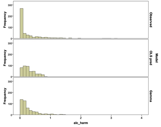
This result may indicate that gamma regression is more appropriate for our purposes than OLS regression, but the fit should be checked directly. The distributions of observed and predicted values in Box 5 show that gamma regression (bottom panel) did a better job of reproducing the original data (top) than did OLS regression (middle). The results are not ideal, however, and the search for a better model might continue.

Zero-inflated negative binomial regression

The methods described so far have been applied to continuous variables, but some outcomes are made up of discrete values, such as responses to a five-point scale, or counts. An often-quoted medical example is the number of admissions to hospital in a year: many people will have no admissions, while a few will have several, giving rise to a positively skewed distribution of integer values. For the purposes of demonstration, we will adapt our continuous outcome so that its distribution is as shown in Box 6.

Faced with such a distribution, researchers may be tempted to recode the variable into two categories, zero (almost 75% of cases) and the rest, and use an analysis which deals with binary outcomes. The risk with this approach is that useful information will be lost when quite different outcomes are lumped together. Zero-inflated negative binomial regression8 provides a way of modelling highly skewed discrete data without combining categories.

In our example, people could be in the zero outcome category because they drink alcohol but do not exhibit harmful drinking patterns, or because they do not drink at all, the latter group inflating the zeroes. In zero-inflated negative binomial regression, independent variables may be considered as possible predictors of whether participants are in the zero-count group, and also of the count — the level of harmful alcohol use in our example. To illustrate, the results in the zero inflation section of Box 7 show that sex helps to discriminate any alcohol use from none (P = 0.022; females are more likely to be in zero category than males, with an odds ratio of 3.5) but, among users, sex does not predict level of use (P = 0.826). In the negative binomial regression section of Box 7, we see that people in the highest anxiety category are more likely to make harmful use of alcohol than those in the lowest category.

The applicability of this model would need to be checked, like that of any other model, but these results demonstrate the usefulness of the distinction between variables which influence the level of an outcome and those which determine whether a zero will be recorded.

Conclusion

One approach to the assumptions that underlie many of the statistical procedures used in medical research is to ignore them; often, this strategy will not result in invalid conclusions. Other strategies are to use non-parametric tests, or to transform outcome variables so that they more nearly conform to the assumptions.

This article has suggested some alternatives: one is to use a resampling technique called bootstrapping to obtain estimates of standard errors from the data themselves; the other is to use models which may be more appropriate than those based on the assumption of normality. Application of these models may lead to additional insights into the data.

Box 1 – Frequency distribution of alc_harm

Box 2 – Shape of the normal distribution

Box 3 – Residuals from an ordinary least squares regression analysis with alc_harm as the outcome variable

Box 5 – Distributions of the observed values of alc_harm, and of the values predicted by ordinary least squares (OLS) regression and gamma regression

Box 6 – Frequency distribution of a discrete version of the outcome variable alc_harm

References

- Lewis-Beck C, Lewis-Beck M. Applied regression: an introduction. 2nd ed. Thousand Oaks, Calif: Sage, 2016.
- Hardy M. Regression with dummy variables. Newbury Park, Calif: Sage, 1993.
- Gibbons J. Nonparametric statistics: an introduction. Thousand Oaks, Calif: Sage, 1992.
- Glass E, Peckham P, Sanders J. Consequences of failure to meet assumptions underlying the fixed effects analyses of variance and covariance. Rev Educ Res 1972; 42: 237-288.
- Mooney C, Duval R. Bootstrapping: a nonparametric approach to statistical inference. Newbury Park, Calif: Sage; 1993.
- Craig JC, Williams GJ, Jones M, et al. The accuracy of clinical symptoms and signs for the diagnosis of serious bacterial infection in young febrile children: prospective cohort study of 15 781 febrile illnesses. BMJ 2010; 340: c1594.
- Hardin J, Hilbe J. Generalized linear models and extensions. 3rd ed. College Station, Tex: Stata Press, 2012.
- Long J, Freese J. Regression models for categorical dependent variables using Stata. 3rd ed. College Station, Tex: Stata Press, 2014.
Provenance: Commissioned; externally peer reviewed.
Interpreting Australian Stillbirth Rate Trends: Implications for Surveillance and Continuous Quality Improvement
Aleena M. Wojcieszek, Kirstine Sketcher-Baker, Christine Andrews, Michael Coory, Imogen Kettle, Melissa Malivoire, David Ellwood, Vicki Flenady
Paracetamol in Pregnancy: Uncertain Evidence, Certain Consequences
David J. Tunnicliffe, Miranda Cumpston, Debra Kennedy, Margie Danchin, Armando Teixeira-Pinto
Fatty Liver Disease in Australia: A Narrative Review on the Epidemiology, Natural History, Prognostication and Management in People With Metabolic Dysfunction
Karl Vaz, Daniel Clayton-Chubb, William W. Kemp, Stuart K. Roberts, Ammar Majeed
Birth prevalence, clinical sequelae, and management of congenital cytomegalovirus infections in Australia, 1999–2023: a national prospective study
Ece Egilmezer, Suzy M Teutsch, Carlos Nunez, Stuart T Hamilton, Adam W Bartlett, Pamela Palasanthiran, Elizabeth J Elliott, William D Rawlinson
The number of cancer‐related deaths that could be attributable to spatial disparities in survival in Australia, 2010–2019: a retrospective population‐based cohort study
Charlotte K Bainomugisa, Jessica Cameron, Paramita Dasgupta, Peter Baade
Mandatory research projects during medical specialist training in Australia and New Zealand
Paulina Stehlik, Caitlin Brandenburg, David A Henry