Understanding statistical hypothesis tests and power

Medical researchers often attempt to understand whether a risk factor is involved in the aetiology of disease or whether an intervention reduces disease; this has been the subject of another article in this series.1 We typically do this by proposing scientific hypotheses from which testable statistical hypotheses can be developed. For example, our scientific hypothesis could be that people with irritable bowel syndrome (IBS) have higher risk of depression compared with those who do not have IBS. A small study might show that one in ten in the control group have depression, compared with two in ten in the IBS group. This might reflect a real difference in the rate of depression between IBS and non-IBS populations, or the difference of one person between groups might simply be the play of chance. An empirical approach to answering this question might be to repeat the study multiple times, with larger numbers, and to look at the consistency of the results. Unfortunately, this is an expensive and time-consuming solution.

In the early 20th century, statisticians proposed different solutions. Fisher (1890–1962) suggested that researchers should start with a statistical hypothesis, commonly in the null form (no difference in incidence of depression in patients with IBS compared with those without depression); the compatibility between the observed data and this null hypothesis could be measured using a P value.2,3 If this was high, one would tend to accept the explanation that the data were consistent with the hypothesis. If it was low, one would tend to reject the hypothesis; no a priori threshold was specified for the P value and it was seen as part of a continuum, with the reader deciding where to set the threshold and how to incorporate other information.3 Neyman and Pearson sought to remove this subjectivity and focus on decision making, suggesting that one should also state an alternate hypothesis — for example, that there is an increased risk of depression in patients with IBS compared with those without depression. The discrepancy between the observed data and what would be expected under the null hypothesis would be calculated (the test statistic) and compared with an a priori threshold. If the test statistic fell below this threshold, the data were judged to be compatible with the null hypothesis. If the test statistic was above the threshold, the null hypothesis would be rejected. These opposing statisticians became embroiled in a long running and bitter feud,4 and we have been left with a legacy that reflects a combination of the two approaches — we frame a null and alternate hypothesis (Neyman and Pearson) but calculate a P value (Fisher). Even recently, the American Statistical Association felt the need to release a statement on the purpose and uses of P values.5

Many clinicians find the null hypothesis counterintuitive, and it is worth exploring why it was adopted. First, it is the simplest hypothesis to test; for example, that any difference between IBS and non-IBS populations in stress observed in our sample is due to chance. Second, it is more efficient to disprove a hypothesis than to prove it; as the philosopher of science Karl Popper argued, falsifiability is a more reliable criterion of truth than verifiability.3,4 It is important to note that rejecting the null hypothesis is not actually specific evidence for the alternate hypothesis, although it is customary to take it as such.

Understanding P values

Consider a clinician who observes that patients with IBS have higher stress scores on the Depression Anxiety Stress Scale6 than patients without IBS. The physician observes that individuals with IBS have a higher mean (x̄) score (mean, 15; SD, 10; n = 20) than non-IBS individuals (mean, 9; SD, 8; n = 42). The scientific hypothesis is that patients with IBS have higher stress scores than those without IBS. The corresponding statistical (null) hypothesis is that there is no difference in stress scores on average between those with and without IBS and the difference observed is simply due to chance. As noted above, the empirical approach would be to repeat this experiment hundreds of times and look for consistency. The beauty of statistics is that it saves us the time and cost of doing this. The P value estimates how likely we are to see this difference, or whether there was no real difference in mean stress scores in the population, or one more extreme, if it was simply the play of chance, without us having to actually do the repeated experiments.

One way of viewing a hypothesis test is as an evaluation of the signal-to-noise ratio. In our example, the signal is the difference between IBS and non-IBS means (15 − 9 = 6 points) and the noise is the uncertainty around that difference between means (reflected through the standard error). In this instance, the appropriate test statistic is an unpaired t test, which is appropriate for the comparison of means of two independent samples of individuals (although there are many different tests appropriate to different scenarios). The t test is calculated as:

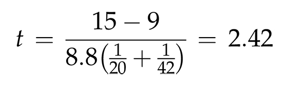
As the numerator (difference between means) increases relative to the denominator (standard error of the difference), we could say that the signal-to-noise ratio increases, increasingly arguing against the null hypothesis and therefore supporting the alternate hypothesis. However, at what point does the ratio become large enough for the clinician to conclude that stress is a feature of IBS? The t value here (2.42) corresponds to a P value of 0.02. The interpretation of this P value is that if we were to repeat the experiment 100 times, and there were truly no difference in the population means, we would expect that two times out of 100 we would see a difference this large or larger. Fisher would leave it to us to decide whether this was rare enough for us to accept our hypothesis of an association, while Neyman and Pearson would say that anything less than 0.05 (five times out of 100), for example, is rare enough to reject the null hypothesis.

Flaws in the argument

Understanding the P value this way makes it clear that we are dealing with probabilities not certainties, so errors are possible. One can falsely reject the null hypothesis, concluding that IBS is associated with higher stress levels when it is not. The chance of this happening is another way to understand the P value and is also known as a type I error. The converse is the probability that there is no real difference between the IBS and non-IBS populations. The opposite error is also possible: accepting the null hypothesis of no association when there actually is an association — this is known as a type II error. The converse is the likelihood that there is a difference between IBS and non-IBS groups, which we rightly conclude by rejecting the null hypothesis — this is also called the power of the study.

The likelihood of making these type I and II errors is partly influenced by our sample size, which is why epidemiologists and statisticians give such importance to calculating a sample size before a study begins. Let us return to our example of the possible association between IBS and stress. After the data have been collected, the hypothesis testing process involves calculating a test statistic. In this case, the unpaired t test is calculated as:

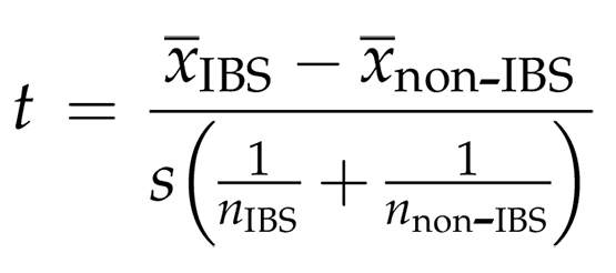
Any quantity in the equation that makes t larger will lead to a smaller P value and increase the likelihood of rejecting the null hypothesis. This means that either the numerator becomes larger or the denominator becomes smaller. The denominator becomes smaller if either the standard deviation (s) is small or the sample size (n) is large. We do not have direct control over standard deviation but we can directly control sample size. Therefore, we might falsely accept the null hypothesis (type II error) either because the standard deviation is large (eg, there is a high degree of measurement error) or because the sample size is small. A red flag for a possible type II error is a clinically meaningful effect size (numerator) but a P value just above our predefined level of statistical significance. Good practice in designing medical studies is to calculate what sample size is required to achieve adequate statistical power (typically ≥ 0.8) at a given level of statistical significance (typically < 0.05), but only if the effect size is large enough to be clinically meaningful. Similarly, it is good practice to report either the a priori sample size calculation or the statistical power available for the sample size achieved.

Conclusion

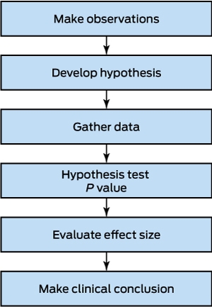
Statistical hypothesis tests require clinical and biological science in their construction and clinical interpretation in applying their results (Box). While they can be viewed as a “black box”, with little or no understanding of their statistical basis, understanding their construction and origins yields important insights into the design of medical studies, including why a prior sample size calculation is important.

Box – The role of statistical hypothesis tests in empirical studies

References

- Jones MP, Walker MM, Attia JA. Understanding statistical principles in correlation, causation and moderation in human disease. Med J Aust 2017; 207: 104-106.
- Greenland S, Senn SJ, Rothman KJ, et al. Statistical tests, p values, confidence intervals and power: a guide to misinterpretations. Eur J Epidemiol 2016; 31: 337-350.
- Sterne JAC, Smith GD. Sifting the evidence — what’s wrong with significance tests? BMJ 2001; 322: 226-231.
- Berger JO. [Could Fisher, Jeffreys and Neyman have agreed on testing?]: Rejoinder. Stat Sci 2003; 18: 28-32.
- Wasserstein RL, Lazar NA. The ASA’s statement on p-values: context, process and purpose. Am Stat 2016; 70: 129-133.
- Crawford JR, Henry JD. The Depression Anxiety Stress Scales (DASS): normative data and latent structure in a large non-clinical sample. Br J Clin Psychol 2003; 42: 111-131.
Provenance: Commissioned; externally peer reviewed.
Interpreting Australian Stillbirth Rate Trends: Implications for Surveillance and Continuous Quality Improvement
Aleena M. Wojcieszek, Kirstine Sketcher-Baker, Christine Andrews, Michael Coory, Imogen Kettle, Melissa Malivoire, David Ellwood, Vicki Flenady
Paracetamol in Pregnancy: Uncertain Evidence, Certain Consequences
David J. Tunnicliffe, Miranda Cumpston, Debra Kennedy, Margie Danchin, Armando Teixeira-Pinto
Fatty Liver Disease in Australia: A Narrative Review on the Epidemiology, Natural History, Prognostication and Management in People With Metabolic Dysfunction
Karl Vaz, Daniel Clayton-Chubb, William W. Kemp, Stuart K. Roberts, Ammar Majeed
Birth prevalence, clinical sequelae, and management of congenital cytomegalovirus infections in Australia, 1999–2023: a national prospective study
Ece Egilmezer, Suzy M Teutsch, Carlos Nunez, Stuart T Hamilton, Adam W Bartlett, Pamela Palasanthiran, Elizabeth J Elliott, William D Rawlinson
The number of cancer‐related deaths that could be attributable to spatial disparities in survival in Australia, 2010–2019: a retrospective population‐based cohort study
Charlotte K Bainomugisa, Jessica Cameron, Paramita Dasgupta, Peter Baade
Mandatory research projects during medical specialist training in Australia and New Zealand
Paulina Stehlik, Caitlin Brandenburg, David A Henry